Ice Cores vs. Plant Stomata Collection

INTRODUCTION

Anyone who has spent any amount of time reviewing climate science literature has probably seen variations of the following chart…

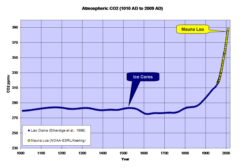
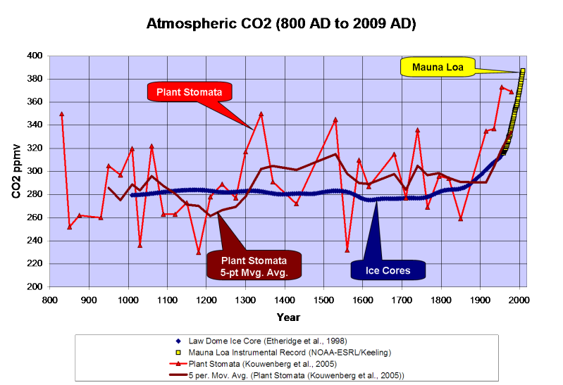
A record of atmospheric CO2 over the last 1,000 years constructed from Antarctic ice cores and the modern instrumental data from the Mauna Loa Observatory suggest that the pre-industrial atmospheric CO2 concentration was a relatively stable ~275ppmv up until the mid 19th Century. Since then, CO2 levels have been climbing rapidly to levels that are often described as unprecedented in the last several hundred thousand to several million years.

Ice core CO2 data are great. Ice cores can yield continuous CO2 records from as far back as 800,000 years ago right on up to the 1970’s. The ice cores also form one of the pillars of Enviromarxist Junk Science: A stable pre-industrial atmospheric CO2 level of ~275ppmv. The Antarctic ice core-derived CO2 estimates are inconsistent with just about every other method of measuring pre-industrial CO2 levels.

Three common ways to estimate pre-industrial atmospheric CO2 concentrations (before instrumental records began in 1959) are:

1) Measuring CO2 content in air bubbles trapped in ice cores.

2) Measuring the density of stomata in plants.

3) GEOCARB (Berner et al., 1991, 1999, 2004): A geological model for the evolution of atmospheric CO2 over the Phanerozoic Eon. This model is derived from “geological, geochemical, biological, and climatological data.” The main drivers being tectonic activity, organic matter burial and continental rock weathering.

ICE CORES

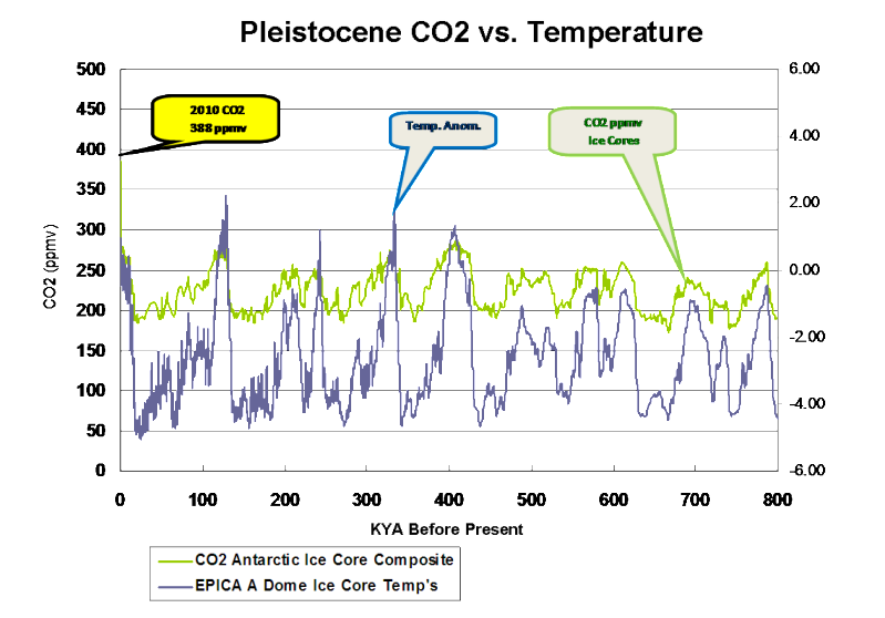
The advantage to the ice core method is that it provides a continuous record of relative CO2 changes going back in time 800,000 years, with a resolution ranging from annual in the shallow section to multi-decadal in the deeper section. Pleistocene-age ice core records seem to indicate a strong correlation between CO2 and temperature; although the delta-CO2 lags behind the delta-T by an average of 800 years…

PLANT STOMATA

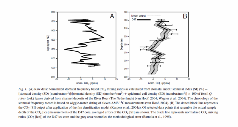
Stomata are microscopic pores found in leaves and the stem epidermis of plants. They are used for gas exchange. The stomatal density in some C3 plants will vary inversely with the concentration of atmospheric CO2. Stomatal density can be empirically tested and calibrated to CO2 changes over the last 60 years in living plants. The advantage to the stomatal data is that the relationship of the Stomatal Index and atmospheric CO2 can be empirically demonstrated…

When stomata-derived CO2 (red) is compared to ice core-derived CO2 (blue), the stomata generally show much more variability in the atmospheric CO2 level and often show levels much higher than the ice cores…

Plant stomata suggest that the pre-industrial CO2 levels were commonly in the 360 to 390ppmv range.

GEOCARB

GEOCARB provides a continuous long-term record of atmospheric CO2 changes; but it is a very low-frequency record…

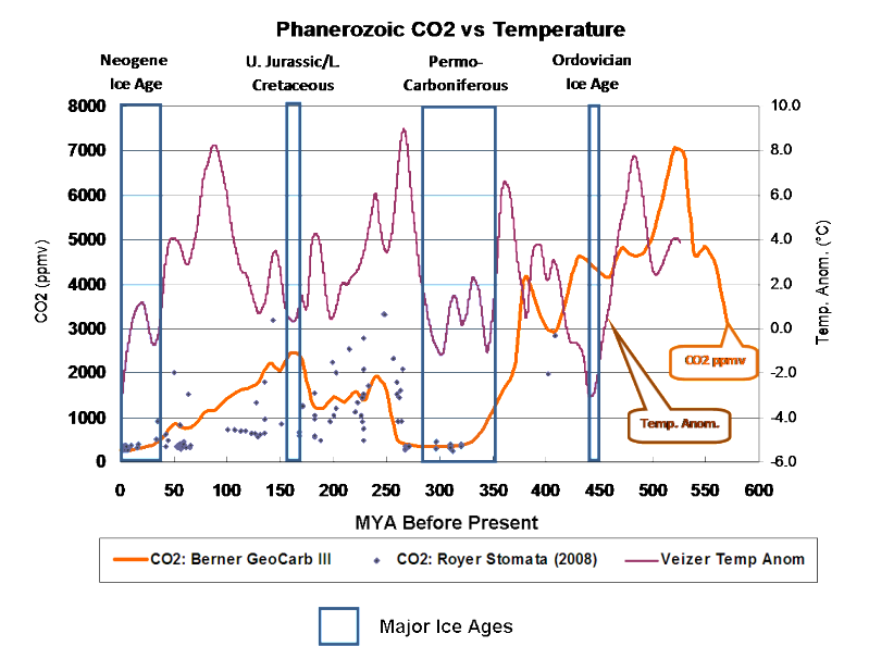
The lack of a long-term correlation between CO2 and temperature is very apparent when GEOCARB is compared to Veizer’s d18O-derived Phanerozoic temperature reconstruction. As can be seen in the figure above, plant stomata indicate a much greater range of CO2 variability; but are in general agreement with the lower frequency GEOCARB model.

DISCUSSION

Ice cores and GEOCARB provide continuous long-term records; while plant stomata records are discontinuous and limited to fossil stomata that can be accurately aged and calibrated to extant plant taxa. GEOCARB yields a very low frequency record, ice cores have better resolution and stomata can yield very high frequency data. Modern CO2 levels are unspectacular according to GEOCARB, unprecedented according to the ice cores and not anomalous according to plant stomata. So which method provides the most accurate reconstruction of past atmospheric CO2?

The problems with the ice core data are 1) the air-age vs. ice-age delta and 2) the effects of burial depth on gas concentrations.

The age of the layers of ice can be fairly easily and accurately determined. The age of the air trapped in the ice is not so easily or accurately determined. Currently the most common method for aging the air is through the use of “firn densification models” (FDM). Firn is more dense than snow; but less dense than ice. As the layers of snow and ice are buried, they are compressed into firn and then ice. The depth at which the pore space in the firn closes off and traps gas can vary greatly… So the delta between the age of the ice and the ago of the air can vary from as little as 30 years to more than 2,000 years.

The EPICA C core has a delta of over 2,000 years. The pores don’t close off until a depth of 99 m, where the ice is 2,424 years old. According to the firn densification model, last year’s air is trapped at that depth in ice that was deposited over 2,000 years ago.

I have a lot of doubts about the accuracy of the FDM method. I somehow doubt that the air at a depth of 99 meters is last year’s air. Gas doesn’t tend to migrate downward through sediment… Being less dense than rock and water, it migrates upward. That’s why oil and gas are almost always a lot older than the rock formations in which they are trapped. I do realize that the contemporaneous atmosphere will permeate down into the ice… But it seems to me that at depth, there would be a mixture of air permeating downward, in situ air, and older air that had migrated upward before the ice fully “lithified”.

A recent study (Van Hoof et al., 2005) demonstrated that the ice core CO2 data essentially represent a low-frequency, century to multi-century moving average of past atmospheric CO2 levels.

Van Hoof et al., 2005. Atmospheric CO2 during the 13th century AD: reconciliation of data from ice core measurements and stomatal frequency analysis. Tellus (2005), 57B, 351–355.

It appears that the ice core data represent a long-term, low-frequency moving average of the atmospheric CO2 concentration; while the stomata yield a high frequency component.

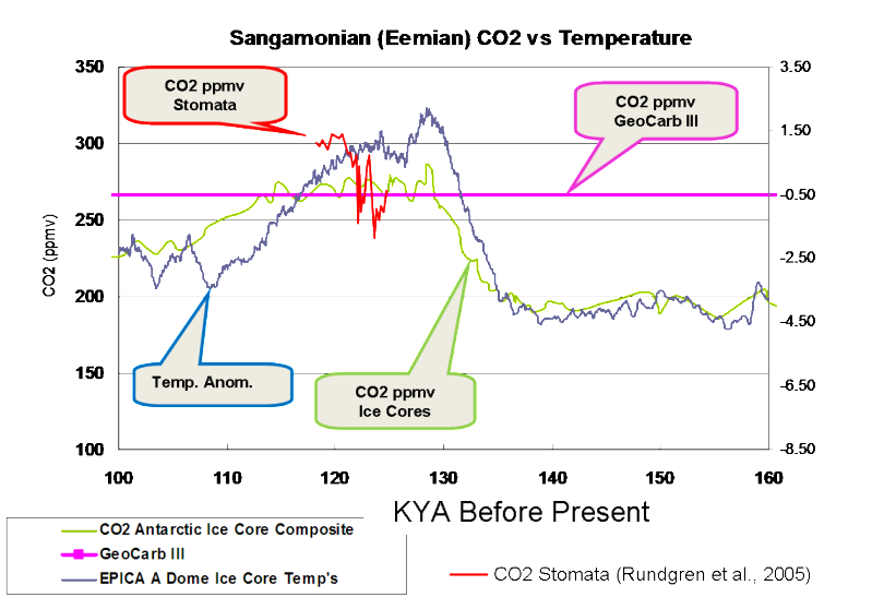
The stomata data routinely show that atmospheric CO2 levels were higher than the ice cores do. Plant stomata data from the previous interglacial (Eemian/Sangamonian) were higher than the ice cores indicate…

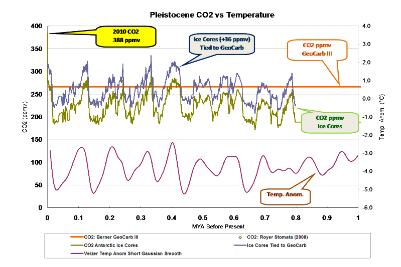
The GEOCARB data also suggest that ice core CO2 data are too low…

The average CO2 level of the Pleistocene ice cores is 36ppmv less than GEOCARB…

Recent satellite data (NASA AIRS) show that atmospheric CO2 levels in the polar regions are significantly less than in lower latitudes…

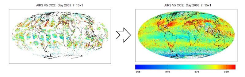
“AIRS can observe the concentration of carbon dioxide in the mid-troposphere, with 15,000 daily observations, pole to pole, all over the globe, with an accuracy of 1 to 2 parts per million and a horizontal surface resolution of 1 by 1 degree. The monthly map at right allows researchers to better observe variations of carbon dioxide at different latitudes and during different seasons. Image credit: NASA” http://www.nasa.gov/topics/earth/agu/airs-images20091214.html

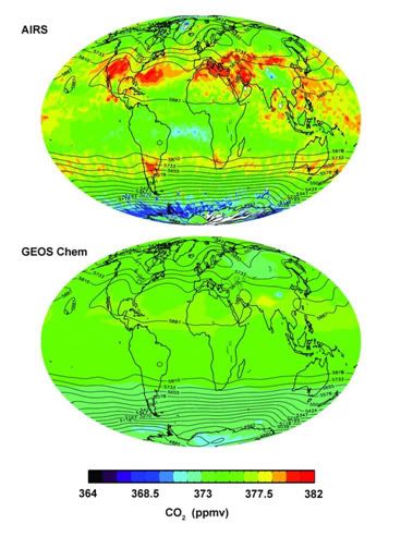
“AIRS data show that carbon dioxide is not well mixed in Earth’s atmosphere, results that have been validated by direct measurements. The belt of carbon dioxide concentration in the southern hemisphere, depicted in red, reaches maximum strength in July-August and minimum strength in December-January. There is a net transfer of carbon dioxide from the northern hemisphere to the southern hemisphere. The northern hemisphere produces three to four times more human produced carbon dioxide than the southern hemisphere. Image credit: NASA” http://www.nasa.gov/topics/earth/agu/airs-images20091214.html

So… The ice core data should be yielding lower CO2 levels than the Mauna Loa Observatory and the plant stomata.

Kouwenberg et al., 2005 found that a “stomatal frequency record based on buried Tsuga heterophylla needles reveals significant centennial-scale atmospheric CO2 fluctuations during the last millennium.”

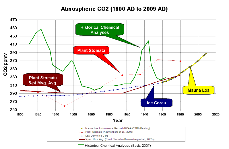
Plant stomata data show much greater variability of atmospheric CO2 over the last 1,000 years than the ice cores and that CO2 levels have often been between 300 and 340ppmv over the last millennium, including a 120ppmv rise from the late 12th Century through the mid 14th Century. The stomata data also indicate higher CO2 levels than the Mauna Loa instrumental record; but a 5-point moving average ties into the instrumental record quite nicely…

A survey of historical chemical analyses (Beck, 2007) shows even more variability in atmospheric CO2 levels than the plant stomata data since 1800…

WHAT DOES IT ALL MEAN?

The current “paradigm” says that atmospheric CO2 has risen from ~275ppmv to 388ppmv since the mid-1800’s as the result of fossil fuel combustion by humans. Increasing CO2 levels are supposedly warming the planet…

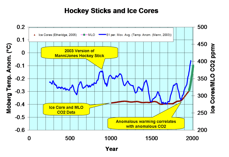
However, if we use Moberg’s (2005) non-Hockey Stick reconstruction, the correlation between CO2 and temperature changes a bit…

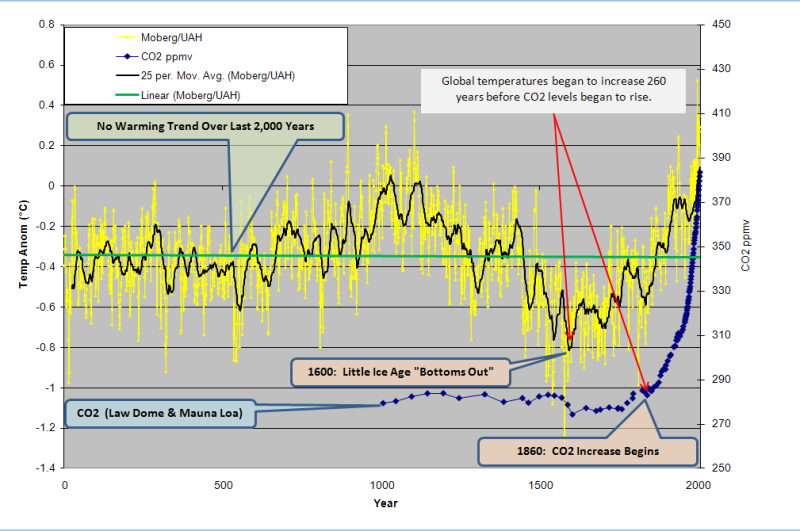
Moberg did a far better job in honoring the low frequency components of the climate signal. Reconstructions like these indicate a far more variable climate over the last 2,000 years than the “Hockey Sticks” do. Moberg also shows that the warm up from the Little Ice Age began in 1600, 260 years before CO2 levels started to rise.

As can be seen below, geologically consistent reconstructions like Moberg and Esper are in far better agreement with “direct” paleotemperature measurements, like Alley’s ice core reconstruction for Central Greenland…

What happens if we use the plant stomata-derived CO2 instead of the ice core data?

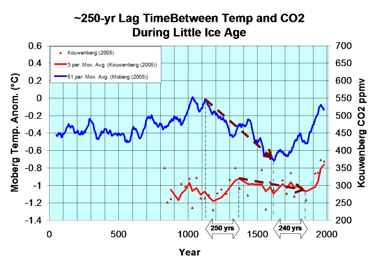
We find that the ~250-year lag time is consistent. CO2 levels peaked 250 years after the Medieval Warm Period peaked and the Little Ice Age cooling began and CO2 bottomed out 240 years after the trough of the Little Ice Age. In a fashion similar to the glacial/interglacial lags in the ice cores, the plant stomata data indicate that CO2 has lagged behind temperature changes by about 250 years over the last millennium. The rise in CO2 that began in 1860 is most likely the result of warming oceans degassing.

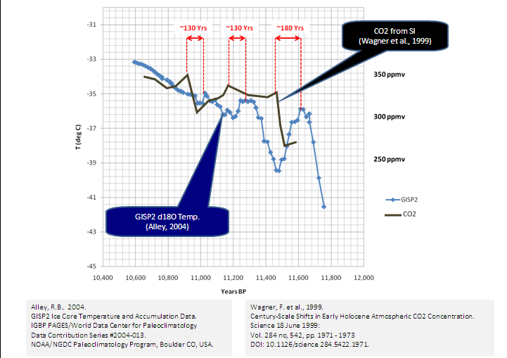
While we don’t have a continuous stomata record over the Holocene, it does appear that a lag time was also present in the early Holocene…

Once dissolved in the deep-ocean, the residence time for carbon atoms can be more than 500 years. So, a 150- to 200-year lag time between the ~1,500-year climate cycle and oceanic CO2 degassing should come as little surprise.

CONCLUSIONS

Ice core data provide a low-frequency estimate of atmospheric CO2 variations of the glacial/interglacial cycles of the Pleistocene. However, the ice cores seriously underestimate the variability of interglacial CO2 levels.
GEOCARB shows that ice cores underestimate the long-term average Pleistocene CO2 level by 36ppmv.
Modern satellite data show that atmospheric CO2 levels in Antarctica are 20 to 30ppmv less than lower latitudes.
Plant stomata data show that ice cores do not resolve past decadal and century scale CO2 variations that were of comparable amplitude and frequency to the rise since 1860.

Thus it is concluded that:

CO2 levels from the Early Holocene through pre-industrial times were highly variable and not stable as the ice cores suggest.
The carbon and climate cycles are coupled in a consistent manner from the Early Holocene to the present day.
The carbon cycle lags behind the climate cycle and thus does not drive the climate cycle.
The lag time is consistent with the hypothesis of a temperature-driven carbon cycle.
The anthropogenic contribution to the carbon cycle since 1860 is minimal and inconsequential.

Note: Unless otherwise indicated, all of the climate reconstructions used in this article are for the Northern Hemisphere.

BIBLIOGRAPHY

Wagner et al., 1999. Century-Scale Shifts in Early Holocene Atmospheric CO2 Concentration. Science 18 June 1999: Vol. 284. no. 5422, pp. 1971 – 1973.

Berner et al., 2001. GEOCARB III: A REVISED MODEL OF ATMOSPHERIC CO2 OVER
PHANEROZOIC TIME. American Journal of Science, Vol. 301, February, 2001, P. 182–204.

Kouwenberg et al., 2004. APPLICATION OF CONIFER NEEDLES IN THE RECONSTRUCTION OF HOLOCENE CO2 LEVELS. PhD Thesis. Laboratory of Palaeobotany and Palynology, University of Utrecht.

Esper et al., 2005. Climate: past ranges and future changes. Quaternary Science Reviews 24 (2005) 2164–2166.

Kouwenberg et al., 2005. Atmospheric CO2 fluctuations during the last millennium reconstructed by stomatal frequency analysis of Tsuga heterophylla needles. GEOLOGY, January 2005.

Van Hoof et al., 2005. Atmospheric CO2 during the 13th century AD: reconciliation of data from ice core measurements and stomatal frequency analysis. Tellus (2005), 57B, 351–355.

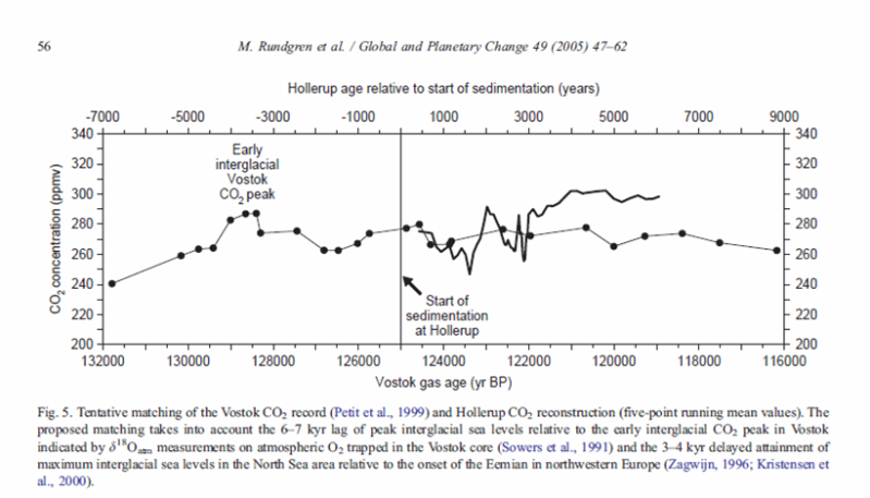
Rundgren et al., 2005. Last interglacial atmospheric CO2 changes from stomatal index data and their relation to climate variations. Global and Planetary Change 49 (2005) 47–62.

Jessen et al., 2005. Abrupt climatic changes and an unstable transition into a late Holocene Thermal Decline: a multiproxy lacustrine record from southern Sweden. J. Quaternary Sci., Vol. 20(4) 349–362 (2005).

Beck, 2007. 180 Years of Atmospheric CO2 Gas Analysis by Chemical Methods. ENERGY & ENVIRONMENT. VOLUME 18 No. 2 2007.

Loulergue et al., 2007. New constraints on the gas age-ice age difference along the EPICA ice cores, 0–50 kyr. Clim. Past, 3, 527–540, 2007.

DATA SOURCES

CO2

Etheridge et al., 1998. Historical CO2 record derived from a spline fit (75 year cutoff) of the Law Dome DSS, DE08, and DE08-2 ice cores.

NOAA-ESRL / Keeling.

Berner, R.A. and Z. Kothavala, 2001. GEOCARB III: A Revised Model of Atmospheric CO2 over Phanerozoic Time, IGBP PAGES/World Data Center for Paleoclimatology Data Contribution Series # 2002-051. NOAA/NGDC Paleoclimatology Program, Boulder CO, USA.

Kouwenberg et al., 2005. Atmospheric CO2 fluctuations during the last millennium reconstructed by stomatal frequency analysis of Tsuga heterophylla needles. GEOLOGY, January 2005.

Lüthi, D., M. Le Floch, B. Bereiter, T. Blunier, J.-M. Barnola, U. Siegenthaler, D. Raynaud, J. Jouzel, H. Fischer, K. Kawamura, and T.F. Stocker. 2008. High-resolution carbon dioxide concentration record 650,000-800,000 years before present. Nature, Vol. 453, pp. 379-382, 15 May 2008. doi:10.1038/nature06949.

Royer, D.L. 2006. CO2-forced climate thresholds during the Phanerozoic. Geochimica et Cosmochimica Acta, Vol. 70, pp. 5665-5675. doi:10.1016/j.gca.2005.11.031.

TEMPERATURE RECONSTRUCTIONS

Moberg, A., et al. 2005. 2,000-Year Northern Hemisphere Temperature Reconstruction. IGBP PAGES/World Data Center for Paleoclimatology Data Contribution Series # 2005-019. NOAA/NGDC Paleoclimatology Program, Boulder CO, USA.

Esper, J., et al., 2003, Northern Hemisphere Extratropical Temperature Reconstruction, IGBP PAGES/World Data Center for Paleoclimatology Data Contribution Series # 2003-036. NOAA/NGDC Paleoclimatology Program, Boulder CO, USA.

Mann, M.E. and P.D. Jones, 2003, 2,000 Year Hemispheric Multi-proxy Temperature Reconstructions, IGBP PAGES/World Data Center for Paleoclimatology Data Contribution Series #2003-051. NOAA/NGDC Paleoclimatology Program, Boulder CO, USA.

Alley, R.B.. 2004. GISP2 Ice Core Temperature and Accumulation Data. IGBP PAGES/World Data Center for Paleoclimatology Data Contribution Series #2004-013. NOAA/NGDC Paleoclimatology Program, Boulder CO, USA.

VEIZER d18O% ISOTOPE DATA. 2004 Update.

Tom Van Hoof, an actual plant physiologist and author of numerous peer-reviewed papers on plant stomata made these comments…

Tom van Hoof on December 28, 2010 at 6:48 am
As one of the “stomata: people and author ofd the cited Tellus paper, I want to draw attention to one of the most interesting outcomes of our research. That is that for the past thousand years the stomata records seem to match with respect to timing to two Antarctic ice core records which are not often cited…. Matching variabilities between ice cores of such resolution has not been achieved yet… well, ice core people claim that they reproduce their flat liners, but if you zoom into detail the small fluxes never match wit respect to timing… The lone fact that stomata data of the USA and Europe have the same timing of a CO2 wiggle which has also been recorded (but with a much lower amplitude) in two Antarctic ice cores is evidence enough that Co2 variability has been larger in the past millennium then assumed. If the variability would have been as small as the ice cores tell us, plant would hav e never ever picked this signal up on two different continents on another hemisphere.

Tom van Hoof on December 28, 2010 at 11:46 pm
@ David Middleton… well actually for the somewhat older stomata data ( I focussed on the past 1000 yrs but my colleages on the whole Holocene) there are Greenland iced-core records which match pretty well… However, we can’t use them for publictions as the ice community officially redrew them as soon as the Antarctic records became available.. they claimed the records are contaminated by too much dust in the ice….

Furthermore I want to mention that we fully understand there are uncertainties with the stomata data. what bothers me is that for our records the scientific community focusses on these uncertainties in exact prediction while all the flaws and errors in ice data are ignored… furthermore it is quite amusing for me as a biologist to read the papers where physicists try to attack the proxies by playing plant physiologist…. I am very surprised the scientific community does not have a very warm welcome for new innovative techniques when those techniques put question marks at established ideas.., I always learned that these discussions are the fundamental backbone for science… therefore my hope that climate science will ever become a fullgrown scientific discipline is lost as long as politics (read funding) keeps intermingling

Tom van Hoof on January 11, 2011 at 8:24 am
To come back on questions about the validity of Stomatal index (read, NOT stomatal density) as a CO2 proxy…

We use an index value between the number of leaf stomata and the number of epidermis cells called the stomatal index instead of just the number of stomata per leafarea as some people tned to do, the reason for thsi is that indeed drought can have an influence on stomatal density, but only through the mechanism on epidermal cell expansion… By using the stomatal index the response of leaf anatomy to changes in water availability are covered, temperature itself has almost no influence on leaf anatomy, only if you would change the annual average temperature 10 of degrees celcius as is done in soem experiments… but this is not comparable with a natural situation… So basically using this index proxy we are pretty sure we are looking at CO2 levels… how big they are is something different… calibration is difficult as it relies on historical CO2 data…

The amount of noise, we choose not to put all sorts of high tech statistical tricks over our data so we are very open about our data, in my opinion noise reduction is possible when more leaves are counted….

Quote:

Ice Core Resolution

The so-called consensus will continue overestimating CO2 forcing until they accept the fact that ice core temperature estimates are at least an order of magnitude of higher resolution than ice core CO2 estimates. The ever-growing volume of peer-reviewed research on the relationship between plant stomata and CO2 will eventually force a paradigm shift.

Wagner et al., 1999. Century-Scale Shifts in Early Holocene Atmospheric CO2 Concentration. Science 18 June 1999: Vol. 284 no. 5422 pp. 1971-1973…

In contrast to conventional ice core estimates of 270 to 280 parts per million by volume (ppmv), the stomatal frequency signal suggests that early Holocene carbon dioxide concentrations were well above 300 ppmv.

[…]

Most of the Holocene ice core records from Antarctica do not have adequate temporal resolution.

[…]

Our results falsify the concept of relatively stabilized Holocene CO2 concentrations of 270 to 280 ppmv until the industrial revolution. SI-based CO2 reconstructions may even suggest that, during the early Holocene, atmospheric CO2 concentrations that were .300 ppmv could have been the rule rather than the exception.

The ice cores cannot resolve CO2 shifts that occur over periods of time shorter than twice the bubble enclosure period. This is basic signal theory. The assertion of a stable pre-industrial 270-280 ppmv is flat-out wrong.

McElwain et al., 2001. Stomatal evidence for a decline in atmospheric CO2 concentration during the Younger Dryas stadial: a comparison with Antarctic ice core records. J. Quaternary Sci., Vol. 17 pp. 21–29. ISSN 0267-8179…

It is possible that a number of the short-term fluctuations recorded using the stomatal methods cannot be detected in ice cores, such as Dome Concordia, with low ice accumulation rates. According to Neftel et al. (1988), CO2 fluctuation with a duration of less than twice the bubble enclosure time (equivalent to approximately 134 calendar yr in the case of Byrd ice and up to 550 calendar yr in Dome Concordia) cannot be detected in the ice or reconstructed by deconvolution.

Not even the highest resolution ice cores, like Law Dome, have adequate resolution to correctly image the MLO instrumental record.

Kouwenberg et al., 2005. Atmospheric CO2 fluctuations during the last millennium reconstructed by stomatal frequency analysis o fTsuga heterophylla needles . Geology; January 2005; v. 33; no. 1; p. 33–36…

The discrepancies between the ice-core and stomatal reconstructions may partially be explained by varying age distributions of the air in the bubbles because of the enclosure time in the firn-ice transition zone. This effect creates a site-specific smoothing of the signal (decades for Dome Summit South [DSS], Law Dome, even more for ice cores at low accumulation sites), as well as a difference in age between the air and surrounding ice, hampering the construction of well-constrained time scales (Trudinger et al., 2003).

Stomatal reconstructions are reproducible over at least the Northern Hemisphere, throughout the Holocene and consistently demonstrate that the pre-industrial natural carbon flux was far more variable than indicated by the ice cores.

Wagner et al., 2004. Reproducibility of Holocene atmospheric CO2 records based on stomatal frequency. Quaternary Science Reviews. 23 (2004) 1947–1954…

The majority of the stomatal frequency-based estimates of CO 2 for the Holocene do not support the widely accepted concept of comparably stable CO2 concentrations throughout the past 11,500 years. To address the critique that these stomatal frequency variations result from local environmental change or methodological insufficiencies, multiple stomatal frequency records were compared for three climatic key periods during the Holocene, namely the Preboreal oscillation, the 8.2 kyr cooling event and the Little Ice Age. The highly comparable fluctuations in the paleo-atmospheric CO2 records, which were obtained from different continents and plant species (deciduous angiosperms as well as conifers) using varying calibration approaches, provide strong evidence for the integrity of leaf-based CO2 quantification.

The Antarctic ice cores lack adequate resolution because the firn densification process acts like a low-pass filter.

Van Hoof et al., 2005. Atmospheric CO2 during the 13th century AD: reconciliation of data from ice core measurements and stomatal frequency analysis. Tellus 57B (2005), 4…

AtmosphericCO2 reconstructions are currently available from direct measurements of air enclosures in Antarctic ice and, alternatively, from stomatal frequency analysis performed on fossil leaves. A period where both methods consistently provide evidence for natural CO2 changes is during the 13th century AD. The results of the two independent methods differ significantly in the amplitude of the estimated CO2 changes (10 ppmv ice versus 34 ppmv stomatal frequency). Here, we compare the stomatal frequency and ice core results by using a firn diffusion model in order to assess the potential influence of smoothing during enclosure on the temporal resolution as well as the amplitude of the CO2 changes. The seemingly large discrepancies between the amplitudes estimated by the contrasting methods diminish when the raw stomatal data are smoothed in an analogous way to the natural smoothing which occurs in the firn.

The derivation of equilibrium climate sensitivity (ECS) to atmospheric CO2 is largely based on Antarctic ice cores. The problem is that the temperature estimates are based on oxygen isotope ratios in the ice itself; while the CO2 estimates are based on gas bubbles trapped in the ice.

The temperature data are of very high resolution. The oxygen isotope ratios are functions of the temperature at the time of snow deposition. The CO2 data are of very low and variable resolution because it takes decades to centuries for the gas bubbles to form. The CO2 values from the ice cores represent average values over many decades to centuries. The temperature values have annual to decadal resolution.

Ice Core Resolution

The highest resolution Antarctic ice core is the DE08 core from Law Dome.

Law Dome DE08 Ice Core: Reconstruction of 1969 AD depositional layer. Modified after Fischer, H. A Short Primer on Ice Core Science. Climate and Environmental Physics, Physics Institute, University of Bern.

The IPCC and so-called scientific consensus assume that it can resolve annual changes in CO2. But it can’t. Each CO2 value represents a roughly 30-yr average and not an annual value.

If you smooth the Mauna Loa instrumental record (red curve) and plant stomata-derived pre-instrumental CO2 (green curve) with a 30-yr filter, they tie into the Law Dome DE08 ice core (light blue curve) quite nicely…

The deeper DSS core (dark blue curve)has a much lower temporal resolution due to its much lower accumulation rate and compaction effects. It is totally useless in resolving century scale shifts, much less decadal shifts.

The IPCC and so-called scientific consensus correctly assume that resolution is dictated by the bubble enclosure period. However, they are incorrect in limiting the bubble enclosure period to the sealing zone. In the case of the core DE08 they assume that they are looking at a signal with a 1 cycle/1 yr frequency, sampled once every 8-10 years. The actual signal has a 1 cycle/30-40 yr frequency, sampled once every 8-10 years.

30-40 ppmv shifts in CO2 over periods less than ~60 years cannot be accurately resolved in the DE08 core. That’s dictated by basic signal theory. Wagner et al., 1999 drew a very hostile response from the so-called scientific consensus. All Dr. Wagner-Cremer did to them, was to falsify one little hypothesis…

In contrast to conventional ice core estimates of 270 to 280 parts per million by volume (ppmv), the stomatal frequency signal suggests that early Holocene carbon dioxide concentrations were well above 300 ppmv.

[…]

Our results falsify the concept of relatively stabilized Holocene CO2 concentrations of 270 to 280 ppmv until the industrial revolution. SI-based CO2 reconstructions may even suggest that, during the early Holocene, atmospheric CO2concentrations that were >300 ppmv could have been the rule rather than the exception (⁠23⁠).

I merged the data from six peer-reviewed papers on stomata-derived CO2 to build this Holocene reconstruction…

Northern Sweden (Finsinger et al., 2009), Northern Spain (Garcia-Amorena, 2008), Southern Sweden (Jessen, 2005), Washington State USA (Kouwenberg, 2004), Netherlands (Wagner et al., 1999), Denmark (Wagner et al., 2002).

The plant stomata pretty well prove that Holocene CO2 levels have frequently been in the 300-350 ppmv range and occasionally above 400 ppmv over the last 10,000 years.

The incorrect estimation of a 3°C ECS to CO2 is almost entirely driven the assumption that preindustrial CO2 levels were in the 270-280 ppmv range, as indicated by the Antarctic ice cores.

The plant stomata data clearly show that preindustrial atmospheric CO2 levels were much higher and far more variable than indicated by Antarctic ice cores. Which means that the rise in atmospheric CO2 since the 1800’s is not particularly anomalous and at least half of it is due to oceanic and biosphere responses to the warm-up from the Little Ice Age.

Kouwenberg concluded that the CO2 maximum ca. 450 AD was a local anomaly because it could not be correlated to a temperature rise in the Mann & Jones, 2003 reconstruction.

As the Earth’s climate continues to not cooperate with their models, the so-called consensus will eventually recognize and acknowledge their fundamental error. Hopefully we won’t have allowed decarbonization zealotry to bankrupt us beforehand.

Until the paradigm shifts, all estimates of the pre-industrial relationship between atmospheric CO2 and temperature derived from Antarctic ice cores will be wrong… Because the ice core temperature and CO2 time series are of vastly different resolutions. And until the “so-called consensus” gets the signal processing right, Professor Nordhaus will continue to get it wrong.

References

Alley, R.B. 2000. The Younger Dryas cold interval as viewed from central Greenland.Quaternary Science Reviews 19:213-226.

Davis, J. C. and G. C. Bohling. The search for patterns in ice-core temperature curves. 2001. Geological Perspectives of Global Climate Change, AAPG Studies in Geology No. 47, Gerhard, L.C., W.E. Harrison,and B.M. Hanson^.

Finsinger, W. and F. Wagner-Cremer. Stomatal-based inference models for reconstruction of atmospheric CO2 concentration: a method assessment using a calibration and validation approach. The Holocene 19,5 (2009) pp. 757–764

Fischer, H. A Short Primer on Ice Core Science. Climate and Environmental Physics, Physics Institute, University of Bern.

Garcıa-Amorena, I., F. Wagner-Cremer, F. Gomez Manzaneque, T. B. van Hoof, S. Garcıa Alvarez, and H. Visscher. 2008. CO2 radiative forcing during the Holocene Thermal Maximum revealed by stomatal frequency of Iberian oak leaves. Biogeosciences Discussions 5, 3945–3964, 2008.

Jessen, C. A., Rundgren, M., Bjorck, S. and Hammarlund, D. 2005. Abrupt climatic changes and an unstable transition into a late Holocene Thermal Decline: a multiproxy lacustrine record from southern Sweden. J. Quaternary Sci., Vol. 20 pp. 349–362. ISSN 0267-8179.

Kaufmann, R. K., H. Kauppi, M. L. Mann, and J. H. Stock (2011), Reconciling anthropogenic climate change with observed temperature 1998-2008, Proceedings of the National Academy of Sciences, PNAS 2011 : 1102467108v1-4.

Kouwenberg, LLR. 2004. Application of conifer needles in the reconstruction of Holocene CO2 levels. PhD Thesis. Laboratory of Palaeobotany and Palynology, University of Utrecht.

Kouwenberg, LLR, Wagner F, Kurschner WM, Visscher H (2005) Atmospheric CO2 fluctuations during the last millennium reconstructed by stomatal frequency analysis of Tsuga heterophylla needles. Geology 33:33–36

Ljungqvist, F.C.2009. Temperature proxy records covering the last two millennia: a tabular and visual overview. Geografiska Annaler: Physical Geography, Vol. 91A, pp. 11-29.

Ljungqvist, F.C. 2010. A new reconstruction of temperature variability in the extra-tropical Northern Hemisphere during the last two millennia. Geografiska Annaler: Physical Geography, Vol. 92 A(3), pp. 339-351, September 2010. DOI: 10.1111/j.1468-0459.2010.00399.x

Mann, M.E., Z. Zhang, M.K. Hughes, R.S. Bradley, S.K. Miller, S. Rutherford, and F. Ni. 2008. Proxy-based reconstructions of hemispheric and global surface temperature variations over the past two millennia. Proceedings of the National Academy of Sciences, Vol. 105, No. 36, September 9, 2008. doi:10.1073/pnas.0805721105

McElwain et al., 2001. Stomatal evidence for a decline in atmospheric CO2 concentration during the Younger Dryas stadial: a comparison with Antarctic ice core records. J. Quaternary Sci., Vol. 17 pp. 21–29. ISSN 0267-8179

Rundgren et al., 2005. Last interglacial atmospheric CO2 changes from stomatal index data and their relation to climate variations. Global and Planetary Change 49 (2005) 47–62.

Van Hoof et al., 2005. Atmospheric CO2 during the 13th century AD: reconciliation of data from ice core measurements and stomatal frequency analysis. Tellus 57B (2005), 4

Wagner F, et al., 1999. Century-scale shifts in Early Holocene CO2 concentration. Science284:1971–1973.

Wagner F, Aaby B, Visscher H, 2002. Rapid atmospheric CO2 changes associated with the 8200-years-B.P. cooling event. Proc Natl Acad Sci USA 99:12011–12014.

Wagner F, Kouwenberg LLR, van Hoof TB, Visscher H, 2004. Reproducibility of Holocene atmospheric CO2 records based on stomatal frequency. Quat Sci Rev 23:1947–1954

A Brief History of Atmospheric Carbon Dioxide Record-Breaking

David Middleton / December 7, 2012

Guest Post by David Middleton

The World Meteorological Organization (Why do I always think of Team America: World Police whenever “World” and “Organization” appear in the same title?) recently announced that atmospheric greenhouse gases had once again set a new record.

Greenhouse gases reach another new record high!

Records are made to be broken

I wonder if the folks at the WMO are aware of the following three facts:

1) The first “record high” CO2 level was set in 1809, at a time when cumulative anthropogenic carbon emissions had yet to exceed the equivalent of 0.2 ppmv CO2?

: Figure 1. The Original CO2 “Hockey Stick.” CO2 emissions data from Oak Ridge National Laboratory’s Carbon Dioxide Information Analysis Center (CDIAC). The emissions (GtC) were divided by 2.13 to obtain ppmv CO2.

2) From 1750 to 1875, atmospheric CO2 rose at ten times the rate of the cumulative anthropogenic emissions…

: Figure 2. Where, oh where, did that CO2 come from?

3) Cumulative anthropogenic emissions didn’t “catch up” to the rise in atmospheric CO2 until 1960…

: Figure 3. It took humans over 100 years to “catch up” to nature.

The emissions were only able to “catch up” because atmospheric CO2 levels stalled at ~312 ppmv from 1940-1955.

The mid-20th century decline in atmospheric CO2

The highest resolution Antarctic ice cores I am aware of come from Law Dome (Etheridge et al., 1998), particularly the DE08 core. Over the past decade, the Law Dome ice core resolution has been improved through denser sampling and the application of frequency enhancing signal processing techniques (Trudinger et el., 2002 and MacFarling Meure et al., 2006). Not surprisingly, the higher resolution data are indicating more variability in preindustrial CO2 levels.

Plant stomata reconstructions (Kouwenberg et al., 2005, Finsinger and Wagner-Cremer, 2009) and contemporary chemical analyses (Beck, 2007) indicate that CO2 levels in the 1930′s to early 1940′s were in the 340 to 400 ppmv range and then declined sharply in the 1950’s. These findings have been rejected by the so-called scientific consensus because this fluctuation is not resolved in Antarctic ice cores. However, MacFarling Meure et al., 2006 found possible evidence of a mid-20th Century CO2 decline in the DE08 ice core…

The stabilization of atmospheric CO2 concentration during the 1940s and 1950s is a notable feature in the ice core record. The new high density measurements confirm this result and show that CO2 concentrations stabilized at 310–312 ppm from ~1940–1955. The CH4 and N2O growth rates also decreased during this period, although the N2O variation is comparable to the measurement uncertainty. Smoothing due to enclosure of air in the ice (about 10 years at DE08) removes high frequency variations from the record, so the true atmospheric variation may have been larger than represented in the ice core air record. Even a decrease in the atmospheric CO2 concentration during the mid-1940s is consistent with the Law Dome record and the air enclosure smoothing, suggesting a large additional sink of ~3.0 PgC yr-1 [Trudinger et al., 2002a]. The d13CO2 record during this time suggests that this additional sink was mostly oceanic and not caused by lower fossil emissions or the terrestrial biosphere [Etheridge et al., 1996; Trudinger et al., 2002a]. The processes that could cause this response are still unknown.

[11] The CO2 stabilization occurred during a shift from persistent El Niño to La Niña conditions [Allan and D’Arrigo, 1999]. This coincided with a warm-cool phase change of the Pacific Decadal Oscillation [Mantua et al., 1997], cooling temperatures [Moberg et al., 2005] and progressively weakening North Atlantic thermohaline circulation [Latif et al., 2004]. The combined effect of these factors on the trace gas budgets is not presently well understood. They may be significant for the atmospheric CO2 concentration if fluxes in areas of carbon uptake, such as the North Pacific Ocean, are enhanced, or if efflux from the tropics is suppressed.

From about 1940 through 1955, approximately 24 billion tons of carbon went straight from the exhaust pipes into the oceans and/or biosphere.

Figure 4. Oh where, oh where did all that carbon go?

If oceanic uptake of CO2 caused ocean acidification, shouldn’t we see some evidence of it? Shouldn’t “a large additional sink of ~3.0 PgC yr-1″ (or more) from ~1940–1955 have left a mark somewhere in the oceans? Maybe dissolved some snails or a reef?

Had atmospheric CO2 simply followed the preindustrial trajectory, it very likely would have reached 315-345 ppmv by 2010…

Figure 5. Natural sources probably account for 40-60% of the rise in atmospheric CO2 since 1750.

Oddly enough, plant stomata-derived CO2 reconstructions indicate that CO2 levels of 315-345 ppmv have not been uncommon throughout the Holocene…

Figure 6. CO2 from plant stomata: Northern Sweden (Finsinger et al., 2009), Northern Spain (Garcia-Amorena, 2008), Southern Sweden (Jessen, 2005), Washington State USA (Kouwenberg, 2004), Netherlands (Wagner et al., 1999), Denmark (Wagner et al., 2002).

So, what on Earth could have driven all of that CO2 variability before humans started burning fossil fuels? Could it possibly have been temperature changes?

CO2 as feedback

When I plot a NH temperature reconstruction (Moberg et al., 2005) along with the Law Dome CO2 record, it sure looks to me as if the CO2 started rising about 100 years after the temperature started rising…

Figure 7. Temperature reconstruction (Moberg et al., 2005) and Law Dome CO2 (MacFarling Meure et al., 2006)

The rise in CO2 from 1842-1945 looks a heck of a lot like the rise in temperature from 1750-1852…

Figure 8. Possible relationship between temperature increase and subsequent CO2 rise.

The correlation is very strong. A calculated CO2 chronology yields a good match to the DE08 ice core and stomata-derived CO2 since 1850. However, it indicates that atmospheric CO2 would have reached ~430 ppmv in the mid-12th century AD.

Figure 9. CO2 calculated from Moberg temperatures (dark blue curve), Law Dome ice cores (magenta curve) and plant stomata (green, light blue and purple squares).

The mid-12th century peak in CO2 is not supported by either the ice cores or the plant stomata. The correlation breaks down before the 1830’s. However, the same break down also happens when CO2 is treated as forcing rather than feedback.

CO2 as forcing

If I directly cross plot CO2 vs. temperature with no lag time, I get a fair correlation with the post DE08 core (>1833) data and no correlation at all with pre-DE08 core (<1833) data…

Figure 10. Temperature and [CO2] have a moderate correlation since ~1833; but no correlation at all before 1833.

If I extrapolate out to about 840 ppmv CO2, I get about 3 °C of warming relative to 275 ppmv. So, I get the same amount of warming for a tripling of preindustrial CO2 that the IPCC says we’ll get with a doubling.

Figure 11. CO2 from the Law Dome DE08 core plotted against Moberg’s NH temperature reconstruction.

Based on this correlation, the equilibrium climate sensitivity to a doubling of preindustrial CO2 is ~1.5 to 2.0 °C. But, the total lack of a correlation in the ice cores older than DE08 is very puzzling.

Ice core resolution and the lack a CO2-temperature coupling before 1833

Could the lack of variability in the older (and deeper) cores have something to do with resolution? The DE08 core is of far higher resolution than pretty well all of the other Antarctic ice cores, including the deeper and older DSS core from Law Dome.

Figure 12. The temporal resolution of ice cores is dictated by the snow accumulation rate.

The amplitude of the CO2 “signal” also appears to be well-correlated with the snow accumulation rate (resolution) of the ice cores…

Figure 13. Accumulation rate vs. CO2 for various ice cores from Antarctica and Greenland.

Could it be that snow accumulation rates significantly lower than 1 m/yr simply can’t resolve century-scale and higher frequency CO2 shifts? Could it also be that the frequency degradation is also attenuating the amplitude of the CO2 “signal”?

If the vast majority of the ice cores older and deeper than DE08 can’t resolve century-scale and higher frequency CO2 shifts, doesn’t it make sense that ice core-derived CO2 and temperature would appear to be poorly coupled over most of the Holocene?

Why is it that the evidence always seems to indicate that the IPCC’s best case scenario is the worst that can happen in the real world?

Brad Plummer’s recent piece in the Washington Post featured a graph that caught my eye…

Figure 14. The IPCC’s mythical scenarios. I think the shaded area represents the greentopian range.

It appears that a “business as usual” (A1FI) will turn Earth into Venus by 2100 AD.

But, what happens if I use real data?

Let’s assume that the atmospheric CO2 level will rise along an exponential trend line until 2100.

Figure 15. CO2 projected to 560 ppmv by 2100.

I get a CO2 level of 560 ppmv, comparable to the IPCC SRES B2 emissions scenario…

Figure 16. IPCC emissions scenarios.

So, business as usual will likely lead to the same CO2 level as an IPCC greentopian scenario. Why am I not surprised?

Assuming all of the warming since 1833 was caused by CO2 (it wasn’t), 560 ppmv will lead to about 1°C of additional warming by the year 2100.

Figure 17. Projected temperature rise derived from Moberg NH temperature reconstruction and Law Dome DE08 ice core CO2.
Projected Temp. Anom. = 2.6142 * ln(CO2) – 15.141

How does this compare with the IPCC’s mythical scenarios? About as expected. The worst case scenario based on actual observations is comparable to the IPCC’s best case, greentopian scenario…

Figure 18. Projected temperature rise derived from Moberg NH temperature reconstruction and Law Dome DE08 ice core CO2 indicates that the IPCC’s 2°C “limit” will not be exceeded.

Conclusions

Atmospheric CO2 concentration records were being broken long before anthropogenic emissions became significant.
Atmospheric CO2 levels were rising much faster than anthropogenic emissions from 1750-1875.
Anthropogenic emissions did not “catch up” to atmospheric CO2 until 1960.
The natural carbon flux is much more variable than the so-called scientific consensus thinks it is.
The equilibrium climate sensitivity (ECS) cannot be more than 2°C and is probably closer to 1°C.
The worst-case scenario based on the evidence is comparable to the IPCC’s most greentopian, best-case scenario.
Ice cores with accumulation rates less than 1m/yr are not useful for ECS estimations.

The ECS derived from the Law Dome DE08 ice core and Moberg’s NH temperature reconstruction assumes that all of the warming since 1833 was due to CO2. We know for a fact that at least half of the warming was due to solar influences and natural climatic oscillations. So the derived 2°C is more likely to be 1°C. Since it is clear that about half of the rise from 275 to 400 ppmv was natural, the anthropogenic component of that 1°C ECS is probably less than 0.7°C.

The lack of a correlation between temperature and CO2 from the start of the Holocene up until 1833 and the fact that the modern CO2 rise outpaced the anthropogenic emissions for about 200 years leads this amateur climate researcher to concluded that CO2 must have been a lot more variable over the last 10,000 years than the Antarctic ice core indicate.

Appendix I: Another Way to Look at the CO2 growth rate

In Figure 15 I used the Excel-calculated exponential trend line to extrapolate the MLO CO2 time series to the end of this century. If I extrapolate the emissions and assume 55% of emissions remain in atmosphere, I get ~702 ppmv by the end of the century, with an additional 0.6°C of warming. A total warming of 2.5°C above “preindustrial.” Even this worse than worst case scenario results in about 1°C less warming than the A1B reference scenario. It falls about mid-way between A1B and the top of the greentopian range.

Appendix II: CO2 Records, the Early Years

Whenever CO2 records are mentioned or breathtaking pronouncements like, “Carbon dioxide at highest level in 800,000 years” are made, I always like to take a look at those “records” in a geological context. The following graphs were generated from Bill Illis’ excellent collection of paleo-climate data.

Greenhouse gases reach another new record high! Or did they? The “Anthropocene” doesn’t look a heck of a lot different than the prior 25 million years… Apart from being a lot colder.

The “Anthropocene’s” CO2 “Hockey Stick” looks more like a needle in a haystack from a geological perspective. And it looks to me as if Earth might be on track to run out of CO2 in about 25 million years.

One of my all-time favorites! Note the total lack of correlation between CO2 and temperature throughout most of the Phanerozoic Eon.

In the following bar chart I grouped CO2 by geologic period. The Cambrian through Cretaceous are drawn from Berner and Kothavala, 2001 (GEOCARB), the Tertiary is from Pagani, et al. 2006 (deep sea sediment cores), the Pleistocene is from Lüthi, et al. 2008 (EPICA C Antarctic ice core), the “Anthropocene” is from NOAA-ESRL (Mauna Loa Observatory) and the CO2 starvation is from Ward et al., 2005.

“Anthropocene” CO2 levels are a lot closer to the C3 plant starvation (Ward et al., 2005) range than they are to most of the prior 540 million years.

[SARC ON] I thought about including Venus on the bar chart; but I would have had to use a logarithmic scale. [SARC OFF]

Appendix III: Plant Stomata-Derived CO2

The catalogue of peer-reviewed papers demonstrating higher and more variable preindustrial CO2 levels is quite impressive and growing. Here are a few highlights:

Wagner et al., 1999. Century-Scale Shifts in Early Holocene Atmospheric CO2 Concentration. Science 18 June 1999: Vol. 284 no. 5422 pp. 1971-1973…

In contrast to conventional ice core estimates of 270 to 280 parts per million by volume (ppmv), the stomatal frequency signal suggests that early Holocene carbon dioxide concentrations were well above 300 ppmv.

[…]

Most of the Holocene ice core records from Antarctica do not have adequate temporal resolution.

[…]

Our results falsify the concept of relatively stabilized Holocene CO2 concentrations of 270 to 280 ppmv until the industrial revolution. SI-based CO2 reconstructions may even suggest that, during the early Holocene, atmospheric CO2 concentrations that were .300 ppmv could have been the rule rather than the exception.

It is possible that a number of the short-term fluctuations recorded using the stomatal methods cannot be detected in ice cores, such as Dome Concordia, with low ice accumulation rates. According to Neftel et al. (1988), CO2 fluctuation with a duration of less than twice the bubble enclosure time (equivalent to approximately 134 calendar yr in the case of Byrd ice and up to 550 calendar yr in Dome Concordia) cannot be detected in the ice or reconstructed by deconvolution.

Not even the highest resolution ice cores, like Law Dome, have adequate resolution to correctly image the MLO instrumental record.

Kouwenberg et al., 2005. Atmospheric CO2 fluctuations during the last millennium reconstructed by stomatal frequency analysis of Tsuga heterophylla needles. Geology; January 2005; v. 33; no. 1; p. 33–36…

The discrepancies between the ice-core and stomatal reconstructions may partially be explained by varying age distributions of the air in the bubbles because of the enclosure time in the firn-ice transition zone. This effect creates a site-specific smoothing of the signal (decades for Dome Summit South [DSS], Law Dome, even more for ice cores at low accumulation sites), as well as a difference in age between the air and surrounding ice, hampering the construction of well-constrained time scales (Trudinger et al., 2003).

Wagner et al., 2004. Reproducibility of Holocene atmospheric CO2 records based on stomatal frequency. Quaternary Science Reviews. 23 (2004) 1947–1954…

The majority of the stomatal frequency-based estimates of CO 2 for the Holocene do not support the widely accepted concept of comparably stable CO2 concentrations throughout the past 11,500 years. To address the critique that these stomatal frequency variations result from local environmental change or methodological insufficiencies, multiple stomatal frequency records were compared for three climatic key periods during the Holocene, namely the Preboreal oscillation, the 8.2 kyr cooling event and the Little Ice Age. The highly comparable fluctuations in the paleo-atmospheric CO2 records, which were obtained from different continents and plant species (deciduous angiosperms as well as conifers) using varying calibration approaches, provide strong evidence for the integrity of leaf-based CO2 quantification.

The Antarctic ice cores lack adequate resolution because the firn densification process acts like a low-pass filter.

Van Hoof et al., 2005. Atmospheric CO2 during the 13th century AD: reconciliation of data from ice core measurements and stomatal frequency analysis. Tellus 57B (2005), 4…

Atmospheric CO2 reconstructions are currently available from direct measurements of air enclosures in Antarctic ice and, alternatively, from stomatal frequency analysis performed on fossil leaves. A period where both methods consistently provide evidence for natural CO2 changes is during the 13th century AD. The results of the two independent methods differ significantly in the amplitude of the estimated CO2 changes (10 ppmv ice versus 34 ppmv stomatal frequency). Here, we compare the stomatal frequency and ice core results by using a firn diffusion model in order to assess the potential influence of smoothing during enclosure on the temporal resolution as well as the amplitude of the CO2 changes. The seemingly large discrepancies between the amplitudes estimated by the contrasting methods diminish when the raw stomatal data are smoothed in an analogous way to the natural smoothing which occurs in the firn.

The highest resolution Antarctic ice core is the DE08 core from Law Dome.

The IPCC and so-called scientific consensus assume that it can resolve annual changes in CO2. But it can’t. Each CO2 value represents a roughly 30-yr average and not an annual value.

The deeper DSS core (dark blue curve) has a much lower temporal resolution due to its much lower accumulation rate and compaction effects. It is totally useless in resolving century scale shifts, much less decadal shifts.

In contrast to conventional ice core estimates of 270 to 280 parts per million by volume (ppmv), the stomatal frequency signal suggests that early Holocene carbon dioxide concentrations were well above 300 ppmv.

[…]

Our results falsify the concept of relatively stabilized Holocene CO2 concentrations of 270 to 280 ppmv until the industrial revolution. SI-based CO2 reconstructions may even suggest that, during the early Holocene, atmospheric CO2 concentrations that were >300 ppmv could have been the rule rather than the exception (⁠23⁠).

The plant stomata pretty well prove that Holocene CO2 levels have frequently been in the 300-350 ppmv range and occasionally above 400 ppmv over the last 10,000 years.

The incorrect estimation of a 3°C ECS to CO2 is almost entirely driven the assumption that preindustrial CO2 levels were in the 270-280 ppmv range, as indicated by the Antarctic ice cores.

Kouwenberg concluded that the CO2 maximum ca. 450 AD was a local anomaly because it could not be correlated to a temperature rise in the Mann & Jones, 2003 reconstruction.

Until the paradigm shifts, all estimates of the pre-industrial relationship between atmospheric CO2 and temperature derived from Antarctic ice cores will be wrong, because the ice core temperature and CO2 time series are of vastly different resolutions. And until the “so-called consensus” gets the signal processing right, they will continue to get it wrong.

References

Anklin, M., J. Schwander, B. Stauffer, J. Tschumi, A. Fuchs, J.M. Barnola, and D. Raynaud. 1997. CO2 record between 40 and 8kyr B.P. from the Greenland Ice Core Project ice core.Journal of Geophysical Research 102:26539-26545.

Barnola et al. 1987. Vostok ice core provides 160,000-year record of atmospheric CO2.
Nature, 329, 408-414.

Berner, R.A. and Z. Kothavala, 2001. GEOCARB III: A Revised Model of Atmospheric CO2 over Phanerozoic Time, American Journal of Science, v.301, pp.182-204, February 2001.

Boden, T.A., G. Marland, and R.J. Andres. 2012. Global, Regional, and National Fossil-Fuel CO₂ Emissions. Carbon Dioxide Information Analysis Center, Oak Ridge National Laboratory, U.S. Department of Energy, Oak Ridge, Tenn., U.S.A. doi 10.3334/CDIAC/00001_V2012

Etheridge, D.M., L.P. Steele, R.L. Langenfelds, R.J. Francey, J.-M. Barnola and V.I. Morgan. 1998. Historical CO₂ records from the Law Dome DE08, DE08-2, and DSS ice cores. In Trends: A Compendium of Data on Global Change. Carbon Dioxide Information Analysis Center, Oak Ridge National Laboratory, U.S. Department of Energy, Oak Ridge, Tenn., U.S.A.

Fischer, H. A Short Primer on Ice Core Science. Climate and Environmental Physics, Physics Institute, University of Bern.

Illis, B. 2009. Searching the PaleoClimate Record for Estimated Correlations: Temperature, CO2 and Sea Level. Watts Up With That?

Indermühle A., T.F. Stocker, F. Joos, H. Fischer, H.J. Smith, M. Wahlen, B. Deck, D. Mastroianni, J. Tschumi, T. Blunier, R. Meyer, B. Stauffer, 1999, Holocene carbon-cycle dynamics based on CO2 trapped in ice at Taylor Dome, Antarctica. Nature 398, 121-126.

Kouwenberg, LLR. 2004. Application of conifer needles in the reconstruction of Holocene CO2 levels. PhD Thesis. Laboratory of Palaeobotany and Palynology, University of Utrecht.

Ljungqvist, F.C.2009. Temperature proxy records covering the last two millennia: a tabular and visual overview. Geografiska Annaler: Physical Geography, Vol. 91A, pp. 11-29.

Lüthi, D., M. Le Floch, B. Bereiter, T. Blunier, J.-M. Barnola, U. Siegenthaler, D. Raynaud, J. Jouzel, H. Fischer, K. Kawamura, and T.F. Stocker. 2008. High-resolution carbon dioxide concentration record 650,000-800,000 years before present. Nature, Vol. 453, pp. 379-382, 15 May 2008. doi:10.1038/nature06949

MacFarling Meure, C., D. Etheridge, C. Trudinger, P. Steele, R. Langenfelds, T. van Ommen, A. Smith, and J. Elkins (2006), Law Dome CO₂, CH₄ and N₂O ice core records extended to 2000 years BP, Geophys. Res. Lett., 33, L14810, doi:10.1029/2006GL026152.

Moberg, A., D.M. Sonechkin, K. Holmgren, N.M. Datsenko and W. Karlén. 2005.
Highly variable Northern Hemisphere temperatures reconstructed from low- and high-resolution proxy data. Nature, Vol. 433, No. 7026, pp. 613-617, 10 February 2005.

Morice, C.P., J.J. Kennedy, N.A. Rayner, P.D. Jones (2011), Quantifying uncertainties in global and regional temperature change using an ensemble of observational estimates: the HadCRUT4 dataset, Journal of Geophysical Research, accepted.

Pagani, M., J.C. Zachos, K.H. Freeman, B. Tipple, and S. Bohaty. 2005. Marked Decline in Atmospheric Carbon Dioxide Concentrations During the Paleogene. Science, Vol. 309, pp. 600-603, 22 July 2005.

Rundgren et al., 2005. Last interglacial atmospheric CO2 changes from stomatal index data and their relation to climate variations. Global and Planetary Change 49 (2005) 47–62.

Smith, H. J., Fischer, H., Mastroianni, D., Deck, B. and Wahlen, M., 1999, Dual modes of the carbon cycle since the Last Glacial Maximum. Nature 400, 248-250.

Trudinger, C. M., I. G. Enting, P. J. Rayner, and R. J. Francey (2002), Kalman filter analysis of ice core data 2. Double deconvolution of CO₂ and δ¹³C measurements, J. Geophys. Res., 107(D20), 4423, doi:10.1029/2001JD001112.

Van Hoof et al., 2005. Atmospheric CO2 during the 13th century AD: reconciliation of data from ice core measurements and stomatal frequency analysis. Tellus 57B (2005), 4

Wagner F, et al., 1999. Century-scale shifts in Early Holocene CO2 concentration. Science284:1971–1973.

Wagner F, Aaby B, Visscher H, 2002. Rapid atmospheric CO2 changes associated with the 8200-years-B.P. cooling event. Proc Natl Acad Sci USA 99:12011–12014.

Wagner F, Kouwenberg LLR, van Hoof TB, Visscher H, 2004. Reproducibility of Holocene atmospheric CO2 records based on stomatal frequency. Quat Sci Rev 23:1947–1954

Ward, J.K., Harris, J.M., Cerling, T.E., Wiedenhoeft, A., Lott, M.J., Dearing, M.-D., Coltrain, J.B. and Ehleringer, J.R. 2005. Carbon starvation in glacial trees recovered from the La Brea tar pits, southern California. Proceedings of the National Academy of Sciences, USA 102: 690-694.

Stomata Notes

Ferdinand Engelbeen says:September 30, 2011 at 8:30 am

[…]

I don’t want to go back to 274 ppmv (LIA), but 280 ppmv during the Medieval Warm Period was not that bad.

[…]

Decadal- centennial- and millennial-scale fluctuations in atmospheric CO2 from 270-360 ppmv have been the norm throughout the Holocene. The natural source-sink ratio is far more variable than indicated by the ice cores. This was occurring long before man ever discovered how to burn things.

Wagner et al., 1999. Century-Scale Shifts in Early Holocene Atmospheric CO2 Concentration. Science 18 June 1999: Vol. 284 no. 5422 pp. 1971-1973…

In contrast to conventional ice core estimates of 270 to 280 parts per million by volume (ppmv), the stomatal frequency signal suggests that early Holocene carbon dioxide concentrations were well above 300 ppmv.

[…]

Most of the Holocene ice core records from Antarctica do not have adequate temporal resolution.

[…]

Our results falsify the concept of relatively stabilized Holocene CO2 concentrations of 270 to 280 ppmv until the industrial revolution. SI-based CO2 reconstructions may even suggest that, during the early Holocene, atmospheric CO2 concentrations that were .300 ppmv could have been the rule rather than the exception.

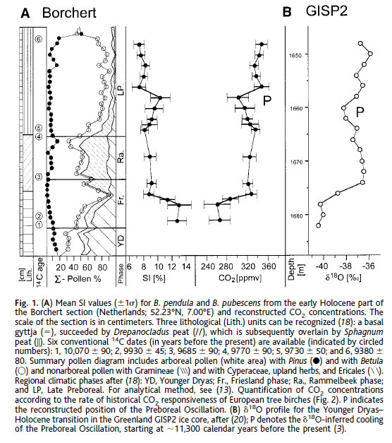
Fig. 1 from Wagner et al., 1999

The ice cores cannot resolve CO2 shifts that occur over periods of time shorter than twice the bubble enclosure period. This is basic Nyquist Sampling Theorem. The assertion of a stable pre-industrial 270-280 ppmv is flat-out wrong.

It is possible that a number of the short-term fluctuations recorded using the stomatal methods cannot be detected in ice cores, such as Dome Concordia, with low ice accumulation rates. According to Neftel et al. (1988), CO2 fluctuation with a duration of less than twice the bubble enclosure time (equivalent to approximately 134 calendar yr in the case of Byrd ice and up to 550 calendar yr in Dome Concordia) cannot be detected in the ice or reconstructed by deconvolution.

Not even the highest resolution ice cores, like Law Dome, have adequate resolution to correctly image the MLO instrumental record.

Kouwenberg et al., 2005. Atmospheric CO2 fluctuations during the last millennium reconstructed by stomatal frequency analysis ofTsuga heterophylla needles . Geology; January 2005; v. 33; no. 1; p. 33–36…

The discrepancies between the ice-core and stomatal reconstructions may partially be explained by varying age distributions of the air in the bubbles because of the enclosure time in the firn-ice transition zone. This effect creates a site-specific smoothing of the signal (decades for Dome Summit South [DSS], Law Dome, even more for ice cores at low accumulation sites), as well as a difference in age between the air and surrounding ice, hampering the construction of well-constrained time scales (Trudinger et al., 2003).

Fig. 3 from Kouwenberg et al., 2005

Wagner et al., 2004. Reproducibility of Holocene atmospheric CO2 records based on stomatal frequency. Quaternary Science Reviews. 23 (2004) 1947–1954…

The majority of the stomatal frequency-based estimates ofCO 2 for the Holocene do not support the widely accepted concept of comparably stable CO2 concentrations throughout the past 11,500 years. To address the critique that these stomatal frequency variations result from local environmental change or methodological insufficiencies, multiple stomatal frequency records were compared for three climatic key periods during the Holocene, namely the Preboreal oscillation, the 8.2 kyr cooling event and the Little Ice Age. The highly comparable fluctuations in the paleo-atmospheric CO2 records, which were obtained from different continents and plant species (deciduous angiosperms as well as conifers) using varying calibration approaches, provide strong evidence for the integrity of leaf-based CO2 quantification.

The Antarctic ice cores lack adequate resolution because the firn densification process acts like a low-pass filter.

Van Hoof et al., 2005. Atmospheric CO2 during the 13th century AD: reconciliation of data from ice core measurements and stomatal frequency analysis. Tellus 57B (2005), 4…

AtmosphericCO2 reconstructions are currently available from direct measurements of air enclosures in Antarctic ice and, alternatively, from stomatal frequency analysis performed on fossil leaves. A period where both methods consistently provide evidence for natural CO2 changes is during the 13th century AD. The results of the two independent methods differ significantly in the amplitude of the estimated CO2 changes (10 ppmv ice versus 34 ppmv stomatal frequency). Here, we compare the stomatal frequency and ice core results by using a firn diffusion model in order to assess the potential influence of smoothing during enclosure on the temporal resolution as well as the amplitude of the CO2 changes. The seemingly large discrepancies between the amplitudes estimated by the contrasting methods diminish when the raw stomatal data are smoothed in an analogous way to the natural smoothing which occurs in the firn.

Any estimate of the pre-industrial relationship between atmospheric CO2 and temperature derived from Antarctic ice cores is wrong… Because the ice core temperature and CO2 time series have vastly different resolutions.

It is physically impossible for Law Dome to have a resolution better than 60 years. The differential between the ice age and gas age is at least 30 years…

Mixing of air from the ice sheet surface to the sealing depth is primarily by molecular diffusion. The rate of air mixing by diffusion in the firn decreases as the density increases and the open porosity decreases with depth. Etheridge et al. (1996) determined the sealing depth at DE08 to be 72 m where the age of the ice is 40±1 years; at DE08-2 to be 72 m depth and 40 years; and at DSS to be 66 m depth and 68 years. For more details on dating the Law Dome ice cores and sealing densities, please refer to Etheridge et al. (1996).

Historical CO2 Records from the Law Dome DE08, DE08-2, and DSS Ice Cores

Ice cores cannot resolve CO2 shifts that occur over time periods less than twice the bubble enclosure time. That is basic Nyquist Sampling Theorem.

At the time the cores were taken, the sealing depth ranged from 66-72 m at an ice age of 40-68 years. None of those cores have the resolution to properly image the MLO instrumental record.

Ferdinand Engelbeen says:

October 1, 2011 at 1:32 am

David Middleton says:

September 30, 2011 at 6:59 pm

You can’t recover higher frequencies than you put into the ground. The Nyquist frequency is equivalent to two-times the bubble enclosure period.

Agreed, but the bubble enclosure period in the high accumulation Law Dome cores is only 8 years starting at 72 m depth. Thus any continuous change of 16 years above the accuracy limits (1.2 ppmv, 1 sigma) can be detected in the ice core. For the lower accumulation third Law Dome core, the closure period is 21 years, thus any frequency of longer than 40 years would be detected. In the case of the MWP-LIA change, the frequency is ~1000 years, thus no problem to detect the change in CO2 between the MWP and LIA, which was about 6 ppmv. That means that it is highly unlikely that the variability seen in stomata data is real, anyway the higher average CO2 levels are impossible, as the ice core data are filtering out the higher frequencies, but filtering doesn’t change the average…

I’m sorry, Ferdinand, but you are totally wrong…

The enclosed air at any depth in the ice has a mean age, (aa), that is younger than the age of the host ice layer (ai), from which the air is extracted. The difference (δa) equals the time (Ts) for the ice layer to reach a depth (ds), where air becomes sealed in the pore space, minus the mean time (Td) for air to mix down the depth. The mean air age is thus

aa = ai + δa = ai + Ts – Td

where ages are dates A.D.

Mixing of air from the ice sheet surface to the sealing depth is primarily by molecular diffusion. The rate of air mixing by diffusion in the firn decreases as the density increases and the open porosity decreases with depth. Etheridge et al. (1996) determined the sealing depth at DE08 to be 72 m where the age of the ice is 40±1 years; at DE08-2 to be 72 m depth and 40 years; and at DSS to be 66 m depth and 68 years. For more details on dating the Law Dome ice cores and sealing densities, please refer to Etheridge et al. (1996).

Historical CO2 Records from the Law Dome DE08, DE08-2, and DSS Ice Cores

Aa = Ai + δa = Ai + Ts – Td

δa = Ts – Td

Aa = Mean air age

Ai = Ice age at extraction depth

Ts = Time for ice to reach sealing depth

Td = Time for air to mix down to sealing depth

DE08 205

Ai= 1939

Aa= 1969

δa= 30

Ts= 40

Td= 10

d= 72

The bubble enclosure time is 4 times the time for the air to mix down to the sealing depth. Every point in the DE08, DE08-2 and DSS cores is approximately a 30-yr moving average of annual CO2 concentrations. The highest frequency recoverable is equivalent to a 30-yr period. The Nyquist frequency at Law Dome is equivalent to a period of 60-yr.

Law Dome cannot resolve CO2 shifts that occur over periods of less than 60 years. That is an absolute immutable fact.

Ferdinand Engelbeen says:

October 2, 2011 at 3:54 pm

David Middleton says:
October 2, 2011 at 6:53 am

David you are confusing between mean gas age of the air enclosed in the ice and gas age distribution within that enclosed air.

At sealing depth of 72 meter, the air is starting to be sealed from the atmosphere. At that moment the average gas age is only 10 years older than in the atmosphere, while the ice age is already 40 years. The gas age distribution at that moment is mainly +/- 3 years, be it with a relative long tail of older gas ages. Then it takes about 8 years to close all bubbles. That means that the average gas age now goes up at the same pace as the ice age, thus the mean gas age now is 18 years and because of less and less sealing bubbles left, the gas age distibution then is less than 8 years + the gas age distribution at sealing start depth, that makes about 11 years for the main age distibution, with relative smaller leads and longer tails of younger and older air, see Fig 11 in:
http://courses.washington.edu/proxies/GHG.pdf

The bubble enclosure time is 4 times the time for the air to mix down to the sealing depth.

Here you are mistaken: there is no bubble enclosure until 72 m depth and all air is fully enclosed at 83 m depth, that is about 8 years (with 1.2 m ice equivalent precipitation at Law Dome). Thus the bubble enclosure time is less than the mix down time of the air in the firn.
The bubble enclosure time and gas age distribution in the bubbles have nothing to do with the mean gas age or ice age or ice age – gas age difference, only with temperature and the static pressure caused by precipitation.

Ferdinand,

You are totally 100% wrong.

Sintering begins when the snow is buried to a depth sufficient to compact its density to 0.55 kg/l (~9 m at DE08). The bubbles begin to close off at ~.70 kg/l (~60 m at DE08) and are completely sealed off at a density of ~0.84 kg/l (72 m at DE08). At the time the core was drilled (1987), the relatively open mixing interval was from the surface down to ~60 m (“1954” ice layer). The sealing interval was from 60-72 m (1954 down to 1946). Even though the sealing interval only spanned 8 ice years, it contained a 30-yr blend of gases because it took that interval ~30 years to be buried to a depth sufficient to achieve sealing density.

At the time of deposition of the “1969” ice layer in the DE-08 core, the top of sealed ice was at an approximate depth of 72 m at the “1929” layer. The sealing interval in 1969 was from the “1937” layer down to the “1929” layer. From the 1969 surface down to the “1937” layer the firn was permeable. During the 10 years that the 1969 air mixed down to the “1939” layer, the 1929-1937 interval sealed completely off.

The air trapped at the “1939” ice layer was a mixture of 1939-1969 air. The mean age of that air was not 1969, as asserted by Etheridge et al.; the mean air age was no younger than 1954. It was actually older than 1954 because the firn/ice becomes less permeable with depth.

Fischer, H. A Short Primer on Ice Core Science. Climate and Environmental Physics, Physics Institute, University of Bern.

Once again, it is physically impossible for the DE08 or DE08-2 cores to resolve CO2 shifts that occur over periods of less than 60 years; and it is impossible for the DSS core to resolve CO2 shifts of shorter duration than 116 years. Below 120 m in the DSS core, the resolution may actually even be much worse than 116 years. There is a pronounce decline in the sampling rate below 120 m. There is a linear decline from 0.74 m/yr to 0.27 m/yr from 116.9 m down to 523.6 m.

The linear nature of the trend means that this is most likely due to compaction, rather than accumulation rate. If the sampling rate decline is due to compaction, it would only have a minimal effect on resolution. If it’s due to accumulation rate, then the resolution below 120 m could be as poor as ~500 years.

Bender, M., T. Sowers & E. Brook. Gases in Ice Cores. Proc. Natl. Acad. Sci. USA. Vol. 94, pp. 8343–8349, August 1997. Colloquium Paper

The most extensive study of the preindustrial CO2 concentration of air and its anthropogenic rise is that of Etheridge et al. (17). Their results are based largely on studies of the DE 08 ice core, from Law Dome, Antarctica (66° 43′ S, 113° 12′ E; elevation 1,250 m). The high accumulation rate, about 1.2 myyr, and warm annual temperature (-19°C) at the site of this core (which causes the closeoff depth to be relatively shallow) allow time to be resolved exceptionally well. Etheridge et al. (17) estimate the gas age–ice age difference to be only 30 yr and the duration of the bubble closeoff process to be 8 yr.

Neftel A, Oeschger H, Staffelbach T, Stauffer B. 1988. CO2 record in the Byrd ice core 50 000–5000 years BP. Nature 331: 609–611.

Because the enclosure process acts as a low pass filter, the CO2 record stored in the ice bubbles of polar ice archive is a smoothed record of the atmospheric CO2 concentration. In the Byrd core the air is enclosed between 60 and 80 m below the surface (m.b.s.) and the duration of the enclosure is ~50 yr during the Holocene.

[…]

Oscillations of the atmospheric CO2 concentration with a period corresponding to twice the enclosure time, 2T would be attenuated to 40% in the ice and would be reinstalled to 82% of the orginal value after the deconvolution procedure. For oscillations corresponding to the duration of the ecclosure time, the percentages would be 8.5% for the CO2 record in ice and 18% for the reconstructed record by the deconvolution procedure. Faster changes are suppressed and cannot be seen in either the ice or reconstructed by deconvolution.

Trudinger, C. M., I. G. Enting, P. J. Rayner, and R. J. Francey (2002), Kalman filter analysis of ice core data 2. Double deconvolution of CO₂ and δ¹³C measurements, J. Geophys. Res., 107(D20), 4423, doi:10.1029/2001JD001112.

JOURNAL OF GEOPHYSICAL RESEARCH, VOL. 107, 4423, 24 PP., 2002
doi:10.1029/2001JD001112

Kalman filter analysis of ice core data 2. Double deconvolution of CO2 and δ13C measurements

C. M. Trudinger

CSIRO Atmospheric Research, Aspendale, Victoria, Australia

I. G. Enting

CSIRO Atmospheric Research, Aspendale, Victoria, Australia

P. J. Rayner

CSIRO Atmospheric Research, Aspendale, Victoria, Australia

R. J. Francey

CSIRO Atmospheric Research, Aspendale, Victoria, Australia

A new method for deconvolving ice core CO₂ and δ¹³CO₂ measurements to estimate net CO₂ uptake by the terrestrial biosphere and the oceans has been developed. The method, which uses the Kalman filter, incorporates statistical analysis into the calculation. This allows a more rigorous analysis of CO₂ variability than the usual deconvolution method. The Kalman filter method estimates uncertainties on the deduced fluxes as part of the calculation. The deconvolution method is applied to the Law Dome CO₂ and δ¹³C ice core record. The calculation suggests that natural variability in CO₂ fluxes may be as large as 1 GtC yr⁻¹ (GtC is gigatonnes carbon, 1 Gt = 10¹⁵ g) on the timescale of just less than a decade. The Law Dome CO₂ measurements show a slight decrease in CO₂ around the 1940s. Analysis with the carbon cycle model and a numerical model of firn processes suggests that about 3 GtC yr⁻¹ uptake (mostly oceanic) is required in the 1940s to match the ice core measurements. The estimates of variation in the terrestrial biospheric flux between 1950 and 1980 from the double deconvolution calculation are in very good agreement with an independent estimate of the global terrestrial flux from a climate-driven ecosystem model.

Published 19 October 2002.

MacFarling Meure, C., D. Etheridge, C. Trudinger, P. Steele, R. Langenfelds, T. van Ommen, A. Smith, and J. Elkins (2006), Law Dome CO₂, CH₄ and N₂O ice core records extended to 2000 years BP, Geophys. Res. Lett., 33, L14810, doi:10.1029/2006GL026152.

GEOPHYSICAL RESEARCH LETTERS, VOL. 33, L14810, 4 PP., 2006
doi:10.1029/2006GL026152

Law Dome CO2, CH4 and N2O ice core records extended to 2000 years BP

C. MacFarling Meure

Marine and Atmospheric Research, Commonwealth Scientific and Industrial Research Organisation, Aspendale, Victoria, Australia

D. Etheridge

Marine and Atmospheric Research, Commonwealth Scientific and Industrial Research Organisation, Aspendale, Victoria, Australia

C. Trudinger

Marine and Atmospheric Research, Commonwealth Scientific and Industrial Research Organisation, Aspendale, Victoria, Australia

P. Steele

Marine and Atmospheric Research, Commonwealth Scientific and Industrial Research Organisation, Aspendale, Victoria, Australia

R. Langenfelds

Marine and Atmospheric Research, Commonwealth Scientific and Industrial Research Organisation, Aspendale, Victoria, Australia

T. van Ommen

Department of the Environment and Heritage, Australian Antarctic Division, and Antarctic Climate and Ecosystems CRC, Hobart, Tasmania, Australia

A. Smith

Australian Nuclear Science and Technology Organisation, Menai, New South Wales, Australia

J. Elkins

NOAA, Earth System Research Laboratory, Boulder, Colorado, USA

New measurements of atmospheric greenhouse gas concentrations in ice from Law Dome, Antarctica reproduce published Law Dome CO₂ and CH₄ records, extend them back to 2000 years BP, and include N₂O. They have very high air age resolution, data density and measurement precision. Firn air measurements span the past 65 years and overlap with the ice core and direct atmospheric observations. Major increases in CO₂, CH₄ and N₂O concentrations during the past 200 years followed a period of relative stability beforehand. Decadal variations during the industrial period include the stabilization of CO₂ and slowing of CH₄ and N₂O growth in the 1940s and 1950s. Variations of up to 10 ppm CO₂, 40 ppb CH₄ and 10 ppb N₂O occurred throughout the preindustrial period. Methane concentrations grew by 100 ppb from AD 0 to 1800, possibly due to early anthropogenic emissions.

Received 26 February 2006; accepted 16 May 2006; published 21 July 2006.

The stabilization of atmospheric CO2 concentration during the 1940s and 1950s is a notable feature in the ice core record. The new high density measurements confirm this result and show that CO2 concentrations stabilized at 310–312 ppm from ~1940–1955. The CH4 and N2O growth rates also decreased during this period, although the N2O variation is comparable to the measurement uncertainty. Smoothing due to enclosure of air in the ice (about 10 years at DE08) removes high frequency variations from the record, so the true atmospheric variation may have been larger than represented in the ice core air record. Even a decrease in the atmospheric CO2 concentration during the mid-1940s is consistent with the Law Dome record and the air enclosure smoothing, suggesting a large additional sink of ~3.0 PgC yr-1 [Trudinger et al., 2002a]. The d13CO2 record during this time suggests that this additional sink was mostly oceanic and not caused by lower fossil emissions or the terrestrial biosphere [Etheridge et al., 1996; Trudinger et al., 2002a]. The processes that could cause this response are still unknown.

[11] The CO2 stabilization occurred during a shift from persistent El Niño to La Niña conditions [Allan and D’Arrigo, 1999]. This coincided with a warm-cool phase change of the Pacific Decadal Oscillation [Mantua et al., 1997], cooling temperatures [Moberg et al., 2005] and progressively weakening North Atlantic thermohaline circulation [Latif et al., 2004]. The combined effect of these factors on the trace gas budgets is not presently well understood. They may be significant for the atmospheric CO2 concentration if fluxes in areas of carbon uptake, such as the North Pacific Ocean, are enhanced, or if efflux from the tropics is suppressed.

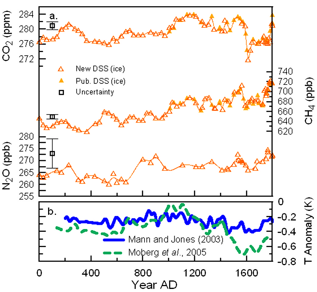
Fig. 2 from MacFarling Meure, et al., 2006

Bandwidth, Sample Rate, and Nyquist Theorem

Bandwidth describes the frequency range in which the input signal can pass through the analog front end with minimal amplitude loss – from the tip of the probe or test fixture to the input of the ADC. Bandwidth is specified as the frequency at which a sinusoidal input signal is attenuated to 70.7% of its original amplitude, also known as the -3 dB point. The following figure shows the typical input response for a 100 MHz high-speed digitizer.

Figure 2

For example, if you input a 1 V, 100 MHz sine wave into high-speed digitizer with a bandwidth of 100 MHz, the signal will be attenuated by the digitizer’s analog input path and the sampled waveform will have an amplitude of approximately 0.7 V.

[+] Enlarge Image
Figure 3

It is recommended that the bandwidth of your digitizer be 3 to 5 times the highest frequency component of interest in the measured signal to capture the signal with minimal amplitude error (bandwidth required = (3 to 5)*frequency of interest). The theoretical amplitude error of a measured signal can be calculated from the ratio of the digitizer’s bandwidth in relation to the input signal frequency (R).

Figure 4

For example, the error in amplitude when measuring a 50 MHz sinusoidal signal with a 100 MHz high-speed digitizer, which yields a ratio of R=2, is approximately 10.5%.

Another important topic related to bandwidth is rise time. The rise time of an input signal is the time for a signal to transition from 10% to 90% of the maximum signal amplitude and is inversely related to bandwidth by the following formula, based on the one pole model, R-C limited input response.

Figure 5

This means that the rise time of a 100 MHz digitizer input path is 3.5 ns. It is recommended that the rise time of the digitizer input path be 1/3 to 1/5 the rise time of the measured signal to capture the signal with minimal rise time error. The theoretical rise time measured (Tr_m) can be calculated from the rise time of the digitizer (Tr_d) and the actual rise time of the input signal (Tr_s).

Figure 6

For example, the rise time measurement when measuring a signal with 12 ns rise time with a 100 MHz digitizer is approximately 12.5 ns.

Nyquist Theorem: Sample rate > 2 * highest frequency component (of interest) of the measured signal

The Nyquist theorem states that a signal must be sampled at a rate greater than twice the highest frequency component of the signal to accurately reconstruct the waveform; otherwise, the high-frequency content will alias at a frequency inside the spectrum of interest (passband). An alias is a false lower frequency component that appears in sampled data acquired at too low a sampling rate. The following figure shows a 5 MHz sine wave digitized by a 6 MS/s ADC. The dotted line indicates the aliased signal recorded by the ADC and is sampled as a 1 MHz signal instead of a 5 MHz signal.

Figure 8: Sine Wave Demonstrating the Nyquist Frequency

The 5 MHz frequency aliases back in the passband, falsely appearing as a 1 MHz sine wave. To prevent aliasing in the passband, you can use a lowpass filter to limit the frequency of the input signal or increase your sampling rate.

Diffusion Confusion

The concept of gas diffusion in ice cores can be a confusing topic.

The age of the layers of ice can be fairly easily and accurately determined. The age of the air trapped in the ice is not so easily or accurately determined. Currently the most common method for aging the air is through the use of “firn densification models” (FDM). Firn is more dense than snow; but less dense than ice. As the layers of snow and ice are buried, they are compressed into firn and then ice. The depth at which the pore space in the firn closes off and traps gas can vary greatly… So the delta between the age of the ice and the age of the air can vary from as little as 30 years to more than 2,000 years.

The DE08 core from Law Dome core has a delta of 30 years. When the core was drilled in 1992 pores didn’t close off until a depth of 83 m, in ice that formed in 1939. According to the firn densification model, air from 1969 was trapped at that depth in ice that was deposited in 1939. It doesn’t seem reasonable to assume that “1969” air was trapped at 83 m in “1939” ice It seems to me that at depth, there would be a mixture of air permeating downward, in situ air, and older air that had migrated upward before the ice fully “lithified.” The air trapped in the 1939 layer should be a blend of air from 1909 to 1969. At the time that the 1939 layer was deposited, the ice crystals above 1909 would not have “lithified” yet. In 1939, the air within the interstitial pore space would be a mixture of 1909 to 1939 air. By the time the 1969 layer was deposited and the 1939 layer “lithified,” the air at the 1939 layer would have been a blend of 1909 to 1969 air.

Here are a schematic diagrams of the two models…

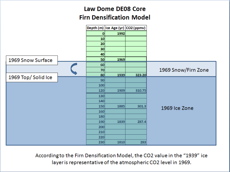
Fig. 1) Schematic diagram of DE08 firn densification model.

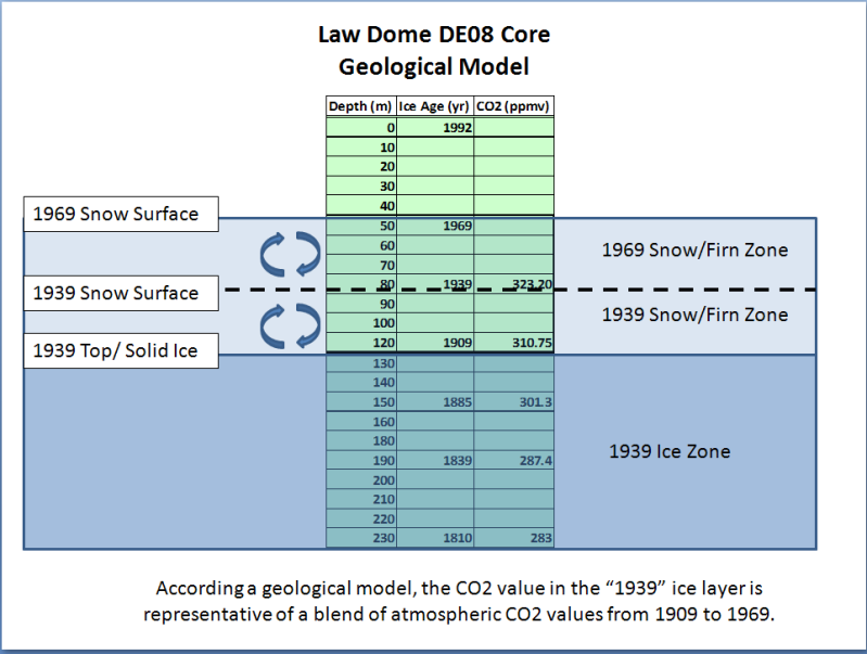
Fig. 2) Schematic diagram of DE08 geological model.

At the time of deposition of the 1939 ice layer, the interval from 1939 down to 1909 would have been composed of unconsolidated ice, snow and firn. A mixture of 1909-1939 air would have permeated the pore space.

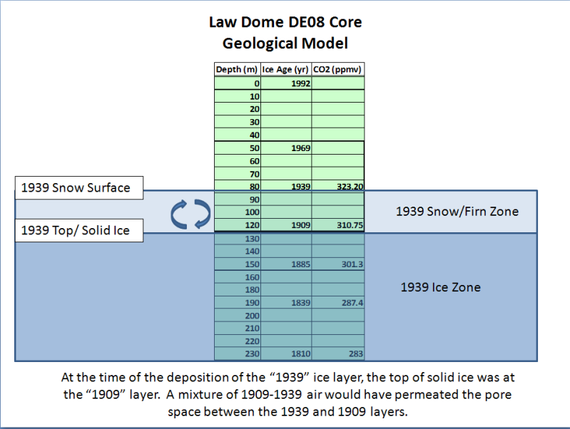
The 1939 layer did not “lithify” until after the depostion of the 1969 layer. The interval from 1969 down to 1939 would have been composed of unconsolidated ice, snow and firn. A mixture of 1939-1969 air would have permeated the pore space.

If the geological model is correct, the CO2 values in the DE08 core are ~60-yr moving averages of atmospheric CO2 levels centered on the ice layer. They are not representative of atmospheric CO2 30 years after the ice layer was deposited as is assumed in the firn densification model.

Plant stomata (Kouwenberg et al.,2005) and contemporary chemical analyses (Beck, 2007) both indicate that CO2 levels in the 1930’s to 1940’s were in the 340 to 400 ppmv range. If CO2 levels had risen in response to the early 20th century warming and then declined in response to the very sharp cooling from the mid 1940’s to mid 1950’s, we should be able to see indications of this in the DE08 core. Using the firn densification model, we do not see evidence of high CO2 levels in the 1930’s to 1940’s. If we use the geological model, we see that the DE08 core is fully consistent with the high CO2 levels in the 1930’s and 1940’s….

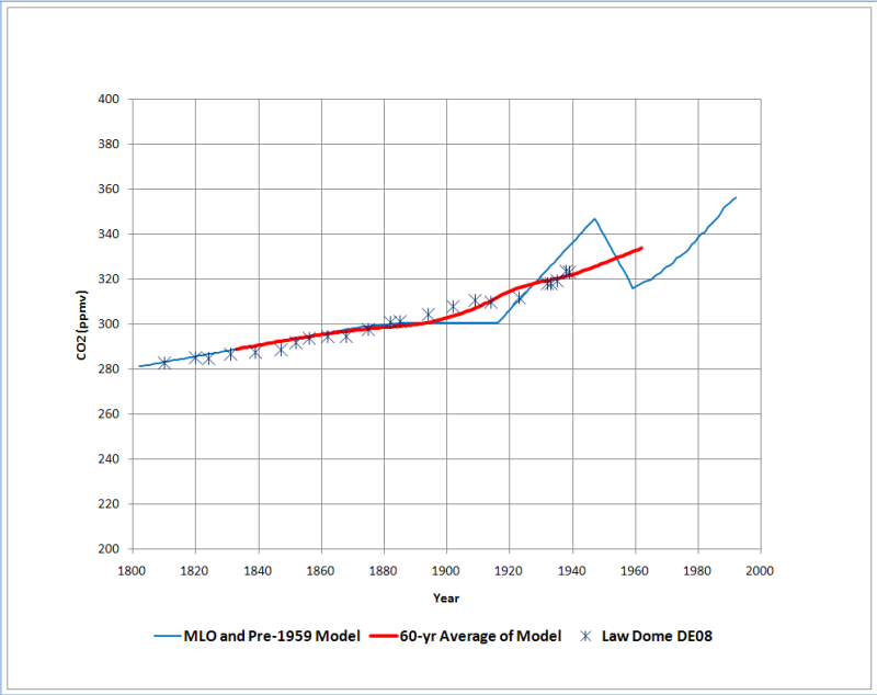
Fig. 5) DE08 Geological model CO2 response.

The pre-1959 model was constructed using the Mauna Loa Co2 data (NOAA/ESRL) I manufactured a CO2 rise in the early 20th century culminating in 1947 at 347 ppmv. Then I calculated a 60-yr running average (heavy red curve). The purple asterisks are the values in the DE08 core plotted against the ice age (not the FD model-derived air age).

The match of the model to the ice core data is pretty striking… Particularly since I threw this together over my lunch hour.

This is one more indication that the Antarctic ice cores are yielding CO2 levels that too low and show too little variation. The amplitude of the CO2 signal is being attenuated in proportion to the accumulation rate of the ice…

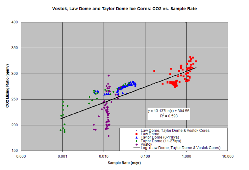
Fig. 6) Sample rate vs. CO2 mixing ratio for three Antarctic ice cores. Sample rate is a proxy for ice accumulation rate.

This relationship is consistent with the findings of van Hoof et al., 2005, which demonstrated that the ice core CO2 data essentially represent a low-frequency, century to multi-century moving average of past atmospheric CO2 levels.

Fig. 7) Van Hoof et al., 2005. Atmospheric CO2 during the 13th century AD: reconciliation of data from ice core measurements and stomatal frequency analysis. Tellus (2005), 57B, 351–355.

References

Barnola, J.M., D. Raynaud, Y. S. Korotkevich† & C. Lorius. 1987. Vostok ice core provides 160,000-year record of atmospheric CO2. Nature 329, 408-414 (1 October 1987) | doi:10.1038/329408a0.

Etheridge, D.M., L.P. Steele, R.L. Langenfelds, R.J. Francey, J.-M. Barnola, and V.I. Morgan. 1996. Natural and anthropogenic changes in atmospheric CO2 over the last 1000 years from air in Antarctic ice and firn. Journal of Geophysical Research 101:4115-4128.

Indermühle, A., T.F. Stocker, F. Joos, H. Fischer, H.J. Smith, M. Wahlen, B. Deck, D. Mastroianni, J. Tschumi, T. Blunier, R. Meyer, B. Stauffer, 1999, Holocene carbon-cycle dynamics based on CO2 trapped in ice at Taylor Dome, Antarctica. Nature 398, 121-126.

Kouwenberg, L., R. Wagner, W.Kürschner, H. Visscher, 2005. Atmospheric CO2 fluctuations during the last millennium reconstructed by stomatal frequency analysis of Tsuga heterophylla needles. GEOLOGY, January 2005.

Van Hoof, T.B., K.A. Kaspers, F. Wagner, R.S.W. van de Wal, W. Kürchner, H. Vissher, 2005. Atmospheric CO2 during the 13th century AD: reconciliation of data from ice core measurements and stomatal frequency analysis. Tellus (2005), 57B, 351–355.

Beck, 2007. 180 Years of Atmospheric CO2 Gas Analysis by Chemical Methods. ENERGY & ENVIRONMENT. VOLUME 18 No. 2 2007.

This entry was posted on March 9, 2015 at 09:15 and is filed under Climate Science, Paleoclimatology. You can follow any responses to this entry through the RSS 2.0 feed. You can leave a response, or trackback from your own site.

Debunk House

Ice Cores vs. Plant Stomata Collection

A Brief History of Atmospheric Carbon Dioxide Record-Breaking

Leave a comment Cancel reply

Debunk House

Ice Cores vs. Plant Stomata Collection

Related

Leave a comment Cancel reply