The Hansen Model: Another very simple disproof of Anthropogenic Global Warming.

Dr. James Hansen is the Director of the Goddard Institute for Space Studies.  Dr. Hansen is right up there with Al Gore, Michael Mann and the Climategate CRU on the list of people helping the UN to swindle the United States and other western democracies out of trillions of dollars through his promotion of the Anthropogenic Global Warming fraud.

Hansen kind of got the ball rolling in 1988 with his publication of a climate model that predicted dire global warming over the next 20 years if mankind did not stop burning fossil fuels… Hansen et al. 1988.

Hansen constructed three scenarios… “Scenario A assumes continued exponential trace gas growth, scenario B assumes a reduced linear linear growth of trace gases, and scenario C assumes a rapid curtailment of trace gas emissions such that the net climate forcing ceases to increase after the year 2000.”

Abstract Hansen et al. 1988 Hansen, J., I. Fung, A. Lacis, D. Rind, Lebedeff, R. Ruedy, G. Russell, and P. Stone, 1988: Global climate changes as forecast by Goddard Institute for Space Studies three-dimensional model. J. Geophys. Res., 93, 9341-9364, doi:10.1029/88JD00231. We use a three-dimensional climate model, the Goddard Institute for Space Studies (GISS) model II with 8° by 10° horizontal resolution, to simulate the global climate effects of time-dependent variations of atmospheric trace gases and aerosols. Horizontal heat transport by the ocean is fixed at values estimated for today’s climate, and the uptake of heat perturbations by the ocean beneath the mixed layer is approximated by vertical diffusion. We make a 100-year control run and perform experiments for three scenarios of atmospheric composition. These experiments begin in 1958 and include measured or estimated changes in atmospheric CO2, CH4, H2O, chlorofluorocarbons (CFCs) and stratospheric aerosols for the period from 1958 to the present. Scenario A assumes continued exponential trace gas growth, scenario B assumes a reduced linear linear growth of trace gases, and scenario C assumes a rapid curtailment of trace gas emissions such that the net climate forcing ceases to increase after the year 2000. Pricipal results from the experiments are as follows: (1) Global warming to the level attained at the peak of the current interglacial and the previous interglacial occurs in all three scenarios; however, there are dramatic differences in the levels of future warming, depending on trace gas growth. (2) The greenhouse warming should be clearly identifiable in the 1990s; the global warming within the next several years is predicted to reach and maintain a level at least three standard deviations above the climatology of the 1950s. (3) Regions where an unambiguous warming appears earliest are low-latitude oceans, China and interior areas in Asia, and ocean areas near Antarctica and the north pole; aspects of the spatial and temporal distribution of predicted warming are clearly model-dependent, implying the possibility of model discrimination by the 1990s and thus improved predictions, if appropriate observations are acquired. (4) The temperature changes are sufficiently large to have major impacts on people and other parts of the biosphere, as shown by computed changes in the frequency of extreme events and comparison with previous climate trends. (5) The model results suggest that some near-term regional climate variations, despite the fixed ocean heat transport which suppresses many possible regional climate fluctuation; for example, during the late 1980s and the 1990s there is a tendency for greater than average warming in the southeastern United States and much of Europe. Principal uncertainties in the predictions involve the equilibrium sensitivity of the model to climate forcing, the assumptions regarding heat uptake and transport by the ocean, and the omission of other less-certain climate forcings.

From Appendix B, pg. 9361 of Hansen’s 1998 paper…

“Specifically, in scenario A CO2 increases as observed by Keeling for the interval 1958-1981 [keeling et al, 1982] and subsequently with a 1.5%/yr growth of the annual increment.”

“In scenario B the growth of the annual increment of CO2 is is reduced from 1.5%/yr today to 1%/yr in 1990, 0.5%/yr in 2000 and 0 in 2010; thus after 2010 is constant, 1.9 ppmv/yr.”

“In scenario C the CO2 growth is the same as scenarios A and B through 1985; between 1985 and 2000 the annual increment is fixed at 1.5 ppmv/yr; after 2000, CO2 ceases to increase, its abundance remaining fixed at 368 ppmv.”

If I take the average annual increment from 1958-1981 and increase it by 1.5% per year until 2008, I get 385.35 ppmv.  The Mauna Loa Observatory’s value for 2008 is 385.57 ppmv.

When I constructed CO2 curves using Hansen’s scenario assumptions and I compare his scenarios to the actual CO2 data recorded since 1988, I get an almost exact match to Scenario “A”…

1988 Hansen Model CO2 vs. Mauna Loa Observatory

Here is a copy of Hansen’s 1988 model with the actual satellite derived temperature (UAH Lower Troposphere) data from Dec. 1979 to November 2009 overlaid…

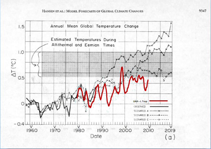
1988 Hansen Model vs. 2009 UAH Lower Troposphere (13-month mvg. avg.)

  Hansen’s scenarios “A” and “B” predicted a temperature anomaly about 1.0°C by 2009. Scenario “C” predicted an anomaly of about 0.7°C by 2009. Since Hansen’s publication, atmospheric CO2 levels have tracked Scenario “A” and CH4 levels have tracked Scenario “C”. Even though CH4 is a more potent greenhouse gas, it accounts for only a tiny fraction of the greenhouse effect:

CO2 is the “Big Kahuna”. Even if CH4 has 20X the greenhouse effect of CO2. 1800 ppb is 0.46% of 390 ppm…20 X 0.46% = 9.2%. At most, CH4 accounts for only about 10% of the greenhouse effect of CO2 in Earth’s current atmosphere.

So, according to Hansen’s 1988 predictions, the global temperature anomaly should be about 90% of the way from Scenario “C” to Scenario “A”… ~0.97°C.   In reality, the global temperature anomaly is about half of what Hansen predicted for a similar rise in greenhouse gases.

The actual warming has been slightly less than Hansen’s Scenario C…

“In scenario C the CO2 growth is the same as scenarios A and B through 1985; between 1985 and 2000 the annual increment is fixed at 1.5 ppmv/yr; after 2000, CO2 ceases to increase, its abundance remaining fixed at 368 ppmv.”

In most branches of science, when experimental results falsify the original hypothesis, scientists discard or modify the original hypothesis.  In Hansen’s case, he just pitches the story with zealotry rarely seen outside of lunatic asylums…

Coal-fired power stations are death factories. Close them

Put oil firm chiefs on trial, says leading climate change scientist

Copenhagen climate change talks must fail, says top scientist

A little known 20 year old climate change prediction by Dr. James Hansen – that failed badly

G-8 Failure Reflects U.S. Failure on Climate Change

Dr. James Hansen of NASA GISS arrested

Jim Hansen calls Cap and Trade the “Temple of Doom”

Is this an example of Jim Hansen’s endorsed “civil disobedience”?

Leading climate scientist: ‘democratic process isn’t working’

Addendum…

In fairness to Dr. Hansen, here’s how his GISTEMP surface temperature data stack up against his model…

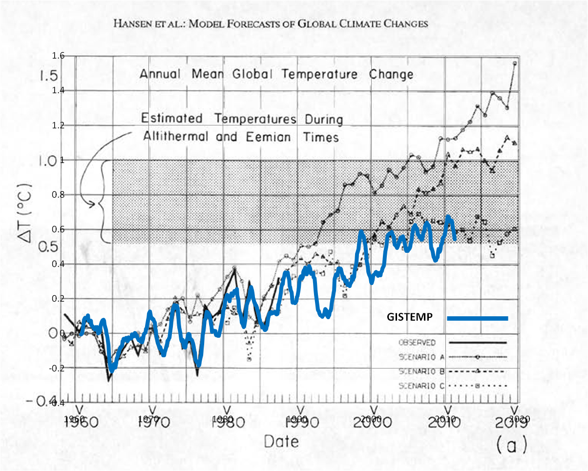
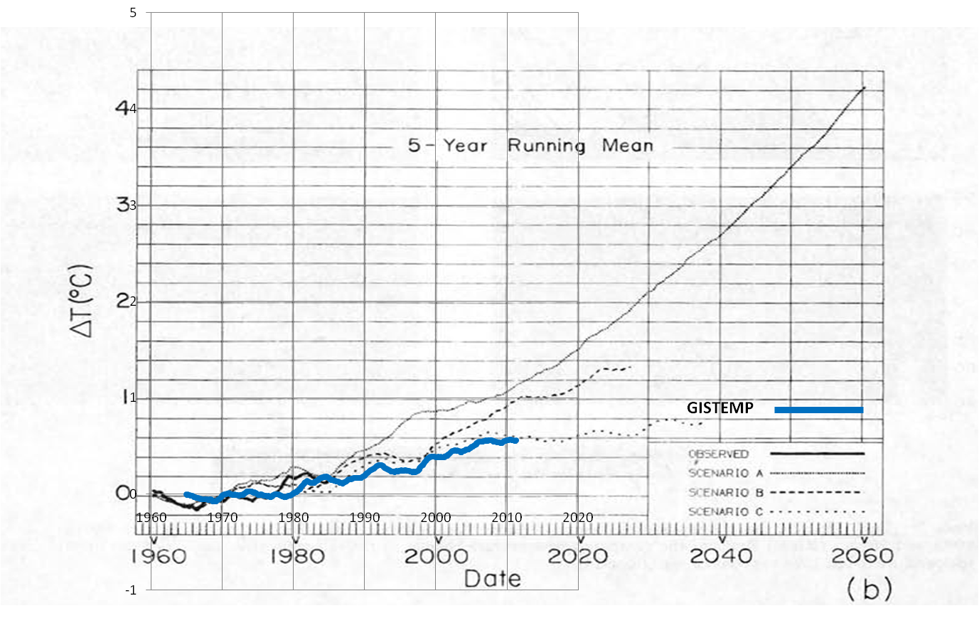
Even GISTEMP is running cold relative to the scenario in which CO2 was held steady at 368 ppmv after the year 2000.