https://www.ncei.noaa.gov/access/monitoring/climate-at-a-glance/statewide/time-series
https://www.ncei.noaa.gov/access/monitoring/historical-palmers/overview
https://www.cjr.org/the_media_today/california_storms_climate_crisis_eric_sorensen.php
https://www.blm.gov/programs/energy-and-minerals/helium/federal-helium-program
https://geology.com/articles/helium/
https://www.usgs.gov/centers/national-minerals-information-center/helium-statistics-and-information
https://pubs.er.usgs.gov/publication/sir20215085
https://www.sciencebase.gov/catalog/item/609e8fe1d34ea221ce3f39e6
MARCH 26, 2018
Source: U.S. Energy Information Administration, Petroleum Supply Monthly, and the Texas Railroad Commission
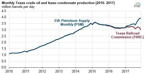
Crude oil and lease condensate production data for Texas, published by EIA in its Petroleum Supply Monthly (PSM) and by the Texas Railroad Commission (TRRC), reflect differences in the treatment of incomplete and lagged data. Data published by state agencies are often incomplete when first published because of a combination of late reporting and processing delays.
TRRC’s most recent report (published March 2018, with estimates through December 2017) is consistent through January 2017 with production estimates in the PSM, but, after January, the two sources diverge. This divergence increases for more recent months: EIA’s most recent production estimates for Texas, published in the PSM on February 28, 2018, show Texas’s crude oil production reaching 3.93 million barrels per day (b/d) in December 2017. TRRC’s values show production at 2.99 million b/d in that same month.
EIA develops state-level production estimates for Texas based on its EIA-914 survey. The EIA-914 survey for oil production was established in 2015, in part to make up for the deficiencies of estimating based on initial state agency reports. EIA monthly oil production volumes are different from the Texas Railroad Commission volumes initially, but as time passes, these differences diminish as TRRC updates and revises its data. EIA’s methodology anticipates and accounts for these expected revisions.
Source: U.S. Energy Information Administration, Petroleum Supply Monthly, and the Texas Railroad Commission
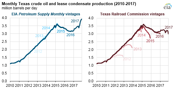
Because EIA’s methodology anticipates revisions, PSM estimates are generally consistent across vintages of data releases, meaning they do not show large revisions as later reports are issued. By contrast, TRRC estimates are consistently revised upward as later reports are issued. The TRRC data are revised upwards over a period of one to two years.
Source: U.S. Energy Information Administration, Petroleum Supply Monthly, and the Texas Railroad Commission
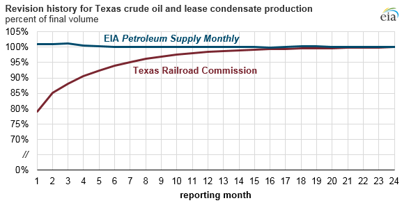
From January 2012 through December 2015, the change in TRRC estimates for any single month has varied from 10% to 31% from month 1 to month 24, with a 12-month average increase of 21%. For the month of December 2017, the TRRC data are 24% below the current EIA estimate.
TRRC’s initial reports tend to be low relative to EIA’s PSM because some oil and natural gas operator reports are placed in a pending file while waiting for other state reporting requirements to be satisfied. Reports may be filed late or have other discrepancies to resolve. Once resolved—generally these resolutions take up to two years—these reports are ultimately included in TRRC’s published reports. On average, TRRC’s published reports are within 95% of their ultimate value after seven months.
Most likely, by late 2019, TRRC’s published production value for December 2017 will be about 3.93 million b/d, consistent with EIA’s most recent PSM estimates. As TRRC continues to revise its data over the next year, we expect the discrepancies observed for the months of 2017 to fall to negligible levels.
Texas is not the only state with incomplete initial monthly data. A full explanation of EIA’s approach for estimating crude oil production in Texas and other states is available in EIA’s methodology report for the PSM.
Principal contributors: Emily Geary, Jess Biercevicz
Tags: crude oil, liquid fuels, oil/petroleum, production/supply, states


Are you now, or have you ever been, a member of the Renewable Energy Dogmatism Party?
Renewable Energy Dogmatism Is Turning the World Red. Just Ask Ukraine and Taiwan
By Patrick Hynes
December 15, 2021In the current day and age, energy security is a prerequisite for national security. When America became energy independent in 2019, it freed us from the political whims of unstable countries. But dogmatic leftists across the world have made it clear that they will sacrifice energy security for their idea of necessary climate policy, seemingly undisturbed by the transfer of that security to communist and authoritarian regimes in China and Russia. As a result, the world might see a Red Revolution before it ever sees a Green one.
While in recent years the US has embraced its liquified natural gas (LNG) boom, European countries steered the other way, ramping down fossil fuel production and increasing their dependence on fossil fuel imports. They have justified this as a “necessary” sacrifice until solar and wind deployment catches up. They are seemingly unconcerned that Russia has become the EU’s largest supplier of fossil fuels, supplying around 40% of the EU’s LNG and coal.
This over-reliance on Russian gas has finally caught up with Europe in the form of a self-inflicted energy crisis. They now rely on Putin to save them through the winter.
[…]
Armed with this newfound political capital, Putin has wasted no time aiming for his most desired prize: Ukraine. A master of political chess, Putin has patiently waited for the right opportunity to continue what he started with Crimea in 2014. Europe’s energy crisis has presented that opportunity, as evident by the buildup of estimated 175,000 troops along the Ukraine border. Since he essentially has the power to turn off the lights this winter for many Western Europeans, he knows that NATO countries will think twice about helping Ukraine, and he is right.
For Taiwan, too, tensions are at an all-time high. Much like with Russia and Ukraine, China does not recognize Taiwan’s independence. The West does, but the West is interested in developing renewable energy, like wind turbines, solar panels, and electric vehicles. The manufacture of such goods requires rare earth minerals. The International Energy Agency estimates that in order to reach net-zero by 2050, “demand for rare earths, primarily used for making EV motors and wind turbines, increases by a factor of ten by 2030.”
Guess who controls nearly 70% of the world’s rare-earths market.
[…]
The West recognizes this issue — it’s far too dependent on China for renewable energy developments — but red tape and lack of expertise make it impossible to compete. Therefore, as the West goes all-in on renewable energy, it will be increasingly dependent on Chinese supply chains wrought with slave labor and carbon-intensive mining. It’s hard not to see Xi Jinping take this as an opportunity to expand China’s global dominance, starting with recapturing Taiwan.
[…]
If Democrats get their way, we’ll end up in the same position as Europe. China will control renewable supply chains, and Russia will control the fossil fuels needed as backup. Energy crises will be more frequent, especially if the weather becomes more erratic with global warming. And communism will spread globally like wildfire. Maybe that is what progressives want.
Patrick Hynes is a Young Voices contributor and an editorial associate at The Conservation Coalition. He also serves as chairman of the Libertarian Party of Washington, DC, and ran for DC’s Delegate to Congress in 2020. Follow him on Twitter @PatrickHynesDC
RealClearEnergy
If Putin seriously wants to seize Ukraine, this winter will probably be his best opportunity. With the US saddled with a dementia-ridden “president” and even less competent “vice president,” the most anti-American administration in US history and a Congress controlled by left-wing zealots for at least the next 12 months and Putin’s ability to turn off Europe’s supply of natural gas on a whim, he is literally in the “catbird seat.” (Yes, I know I just wrote that Putin is literally in an idiomatic phrase.) That said, why would Putin risk triggering World War III? It’s not that there’s a long history of perceived weakness among Western democracies triggering wars in the past…

While we are heavily dependent on Red China for “renewable supply chains,” they are dependent on imported coal, LNG and oil. While that might deter Red China from moving on Taiwan, unless they also militarily enforce the claim that the entire South China Sea is part of their territorial waters/
Red China’s claim was ruled invalid under the United Nations Convention on the Law of the Sea by the Permanent Court of Arbitration in The Hague.
Beijing ignored the ruling.
This EIA analysis was published in 2013.
SOUTH CHINA SEA
Overview
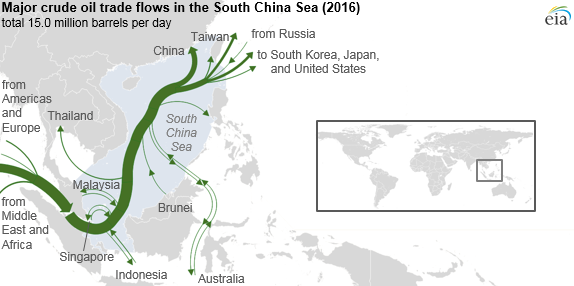
The South China Sea is a critical world trade route and a potential source of hydrocarbons, particularly natural gas, with competing claims of ownership over the sea and its resources.
Stretching from Singapore and the Strait of Malacca in the southwest to the Strait of Taiwan in the northeast, the South China Sea is one of the most important trade routes in the world. The sea is rich in resources and holds significant strategic and political importance.
The area includes several hundred small islands, rocks, and reefs, with the majority located in the Paracel and Spratly Island chains. Many of these islands are partially submerged land masses unsuitable for habitation and are little more than shipping hazards. For example, the total land area of the Spratly Islands encompasses less than 3 square miles.
Several of the countries bordering the sea declare ownership of the islands to claim the surrounding sea and its resources. The Gulf of Thailand borders the South China Sea, and although technically not part of it, disputes surround ownership of that Gulf and its resources as well.
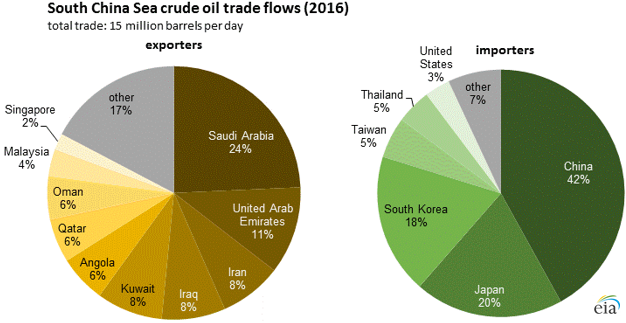
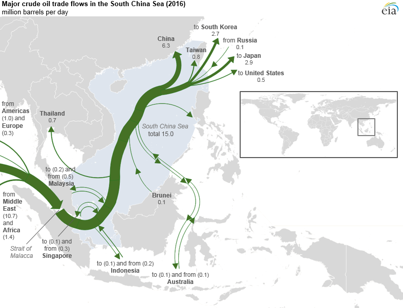
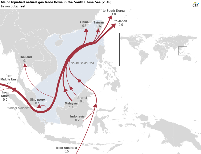
Asia’s robust economic growth boosts demand for energy in the region. The U.S. Energy Information Administration (EIA) projects total liquid fuels consumption in Asian countries outside the Organization for Economic Cooperation and Development (OECD) to rise at an annual growth rate of 2.6 percent, growing from around 20 percent of world consumption in 2008 to over 30 percent of world consumption by 2035. Similarly, non-OECD Asia natural gas consumption grows by 3.9 percent annually, from 10 percent of world gas consumption in 2008 to 19 percent by 2035. EIA expects China to account for 43 percent of that growth.
With Southeast Asian domestic oil production projected to stay flat or decline as consumption rises, the region’s countries will look to new sources of energy to meet domestic demand. China in particular promotes the use of natural gas as a preferred energy source and set an ambitious target of increasing the share of natural gas in its energy mix from 3 percent to 10 percent by 2020. The South China Sea offers the potential for significant natural gas discoveries, creating an incentive to secure larger parts of the area for domestic production.
[…]
EIA
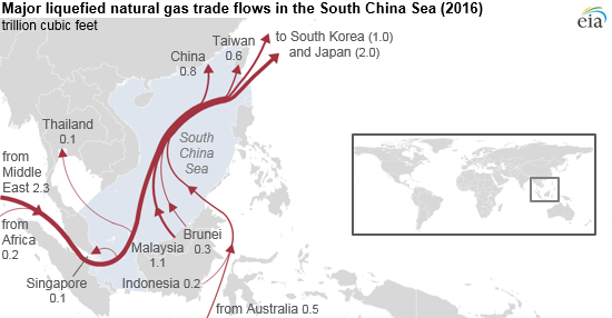
Control of the South China Sea would secure Red China’s oil & LNG imports and enable them to shut off the supply of oil & LNG to Japan, South Korea and Taiwan.

Among the US Navy’s primary missions are Freedom of Navigation Operations (FONOPS), heavily focused on the South China Sea.
7th Fleet Conducts Freedom of Navigation Operation
08 September 2021
From U.S. 7th Fleet Public AffairsOn Sept. 8, USS Benfold (DDG 65) asserted navigational rights and freedoms in the Spratly Islands, consistent with international law. This freedom of navigation operation (“FONOP”) upheld the rights, freedoms, and lawful uses of the sea. USS Benfold demonstrated that Mischief Reef, a low-tide elevation in its natural state, is not entitled to a territorial sea under international law.
[…]
U.S. forces routinely conduct freedom of navigation assertions throughout the world. All of our operations are designed to be conducted in accordance with international law and demonstrate that the United States will fly, sail, and operate wherever international law allows—regardless of the location of excessive maritime claims and regardless of current events.
The United States upholds freedom of navigation as a principle. The Freedom of Navigation Program’s missions are peaceful and conducted without bias for or against any particular country. These missions are rule-of-law based and demonstrate our commitment to upholding the rights, freedoms, and lawful uses of the sea and airspace guaranteed to all nations.
Freedom of navigation operations in the South China Sea are a part of daily operations of U.S. military forces throughout the region.
US Navy
The only forward deployed aircraft carrier in the Western Pacific, CVN 71 USS Theodore Roosevelt was knocked out of action by COVID-19, shortly after Red China unleashed it on the rest of the world… Coincidence?
While I seriously doubt that the two nations who suffered most horribly during World War II would intentional start World War III, why does this remind me of the 1930’s? Substitute Russia for Nazi Germany and Red China for Imperial Japan, toss in a healthy dose of western weakness… and the similarities are eerie.
Anyway, I think it’s time for The Kinks...
‘Cause there’s a red, under my bed
Ray Davies, 1981
And there’s a little yellow man in my head
And there’s a true blue inside of me

