Ocean Acidification: Chicken Little Strikes Again

 

Introduction 

As global warming morphs into climate change and anthropogenic CO2 emissions give way to the Sun, the stars and our oceans as the primary drivers of climate change, environmental extremists like Al Gore are raising a new CO2-driven ecological disaster scenario to hysterical levels: Ocean acidification.   Claims have been made that oceanic pH levels have declined from ~8.2 to ~8.1 since the mid-1700’s.  This pH decline (acidification) has been attributed to anthropogenic CO2 emissions – This should come as no surprise because the pH estimates are largely derived from atmospheric CO2 concentrations (Orr et al., 2005).  It has also been postulated that anthropogenic CO2 emissions will force an additional 0.7 unit decline in oceanic pH by the year 2100 (Caldeira et al., 2003).

Alarmist organizations like the National Resources Defense Council are hard at work extrapolating these oceanic pH model predictions into ecological nightmares…

Scientists predict the Arctic will become corrosive to some shelled organisms within a few decades, and the Antarctic by mid-century. This is pure chemistry; the vagaries of climate do not apply to this forecast.

OA is expected to impact commercial fisheries worldwide, threatening a food source for hundreds of millions of people  as well as a multi-billion dollar industry. In the United States alone, ocean-related tourism, recreation and fishing are responsible for more than 2 million jobs.

Shellfish will be affected directly, thus impacting finfish who feed on them. For example, pteropods—tiny marine snails that are particularly sensitive to rises in acidity— comprise 60 percent of the diet for Alaska’s juvenile pink salmon. And this affects diets farther up the food chain, as a diminished salmon population would lead to less fish on our tables.

Coral reefs will be especially hard hit by ocean acidification. As ocean acidity rises, corals will begin to erode faster than they can grow, and reef structures will be lost worldwide. Scientists predict that by the time atmospheric CO2 reaches 560 parts per million (a level which could happen which could happen by mid-century; we are currently nearing 400 ppm), coral reefs will cease to grow and even begin to dissolve. Areas that depend on healthy coral reefs for food, shoreline protection, and lucrative tourism industries will be profoundly impacted by their loss.

This sounds like a serious threat… As have all of the other alarmist clarion calls to halt capitalism in the name of the most recent environmental causes célèbres.   Just to be fair, before pitching Ocean Acidification into the dustbin of junk science along with Anthropogenic Global Warming, let’s look at the science.

The answers to the following questions will tell us whether or not CO2-driven ocean acidification is a genuine scientific concern: 

1. Is atmospheric CO2 acidifying the oceans?
2. Is there any evidence that reefs and other marine calcifers have been damaged by CO2-driven ocean acidification and/or global warming?
3. Does the geological record support the oceanic acidification hypothesis?  

 

 Is atmospheric CO2 acidifying the oceans?

Before we can answer this question, we have to understand a bit about how the oceans make limestone and other carbonate rocks.   The Carbonate Compensation Depth (CCD or Lysocline) is the depth at which carbonate shells dissolve faster than they accumulate. That depth is primarily determined by several factors…

-Water temperature
-Depth (pressure)
-CO2 concentration
-pH (high pH values aid in carbonate preservation)
-Amount of carbonate sediment supply
-Amount of terrigenous sediment supply

Calcium carbonate solubility increases with increasing carbon dioxide content, lower temperatures, and increasing pressure.

SOURCE

What evidence do we have that the lysocline or CCD has been becoming shallower or that the oceans have been acidifying over the last 250 years?   The answer is: Almost none.

From Pelejero et al., 2005…

The actual trend and range of natural variability in oceanic pH remains largely unknown, yet it is crucial to understand the possible consequences of acidification on marine ecosystems. A reliable proxy record is needed to assess long-term trends and variability in seawater pH. Instrumental records of the seawater CO₂ system, such as those collected at the Hawaii Ocean Time Series Station, which only commenced in 1989 (12), are short. In this Report, we present a reconstruction of seawater pH spanning the last three centuries, based on the boron isotopic composition ( ¹¹B) (13) of a long-lived massive coral (Porites) from Flinders Reef in the western Coral Sea…

[…]

Fig1) Pelejero et al., 2005, Fig. 2. Record of Flinders Reef coral 11B, reconstructed oceanic pH, aragonite saturation state, PDO and IPO indices, and coral calcification parameters. (A) Flinders Reef coral 11B as a proxy for surface-ocean pH (24); 11B measurements for all 5-year intervals are available in table S1. (B) Indices of the PDO (28, 39) and the IPO (27) averaged over the same 5-year intervals as the coral pH data. Gray curves in panels (A) and (B) are the outputs of Gaussian filtering of coral pH and IPO values, respectively, at a frequency of 0.02 ± 0.01 year–1, which represent the 1/50-year component of the pH variation (fig. S2). (C) Comparison of high-resolution coral Sr/Ca (plotted to identify the seasonal cycle of SST) (32), 11B-derived pH, and wind speed recorded at the Willis Island meteorological station (data from the Australian Bureau of Meteorology) (40). Note the covariation of wind speed and seawater pH; strong winds generally occur at times of high pH, and weak winds generally occur at times of low pH. All high-resolution 11B measurements are available in table S2. (D) Aragonite saturation state, , where is the stoichiometric solubility product of aragonite, calculated from our reconstructed pH assuming constant alkalinity (24). (E) Coral extension and calcification rates obtained from coral density measured by gamma ray densitometry (38).

[…]

Although the lowest ¹¹B value for the entire record corresponds to the 5-year average around 1988 [23.0 per mil ( ), 7.91 pH units; Fig. 2A and table S1], there is no notable trend toward lower ¹¹B values. The dominant feature of the coral ¹¹B record is a clear interdecadal oscillation of pH, with ¹¹B values ranging between 23 and 25 (7.9 and 8.2 pH units; Fig. 2A). Spectral analysis of the coral pH record demonstrates a substantial cyclicity of about 50 years (Fig. 2A and fig. S2). Moreover, the variation in pH is synchronous with the Interdecadal Pacific Oscillation (IPO) (27), the Pacific-wide equivalent of the Pacific Decadal Oscillation (PDO) (28), which is also well represented by a 50- to 70-year cyclicity (29) (Fig. 2B and fig. S2). The IPO is well represented by a spatial pattern of sea surface temperature (SST) anomalies over the Pacific Ocean, such that the index is positive when the equatorial Pacific is warm and the southwest Pacific and central North Pacific are cold. This pattern of interdecadal climate variability shares similarities with the El Niño-Southern Oscillation (ENSO), with periods of positive and negative IPO values displaying climatic patterns similar to El Niño and La Niña, respectively (30, 31).

Rather than finding a secular trend of declining pH (ocean acidification), Pelejero et al. found that oceanic pH changes cyclically along with the Pacific Decadal Oscillation and El Niño/La Niña cycle.  So there really is no solid evidence that the oceans have been acidifying since mankind started to burn fossil fuels.

Is there any evidence that reefs and other marine calcifers have been damaged by CO2-driven ocean acidification and/or global warming?

Using the data from Pelejero et al., 2005, I found no correlation between pH and reef calcification rates…

Fig. 2) Flinders Reef: Calcification Rate vs. pH (Pelejero et al., 2005)

 

 A plot of CO2 vs pH from the Flinders Reef dataset shows no statistically significant correlation between atmospheric CO2 and pH from 1788-1988…

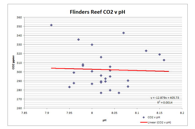
Fig. 3) Fliners Reef pH (Pelejero et al., 2005) vs atmospheric CO2

 

On top of that… There is solid evidence that elevated atmospheric CO2 levels have actually caused carbonate deposition to increase over the last 220 years (Iglesias-Rodriguez et al., 2008)…

Fig. 4) Iglesias-Rodriguez et al., 2008, Fig. 4. Average mass of CaCO3 per coccolith in core RAPID 21-12-B and atmospheric CO2. The average mass of CaCO3 per coccolith in core RAPID 21-12-B (open circles) increased from 1.08 x 10–11 to 1.55 x 10–11 g between 1780 and the modern day, with an accelerated increase over recent decades. The increase in average pre="average ">coccolith mass correlates with rising atmospheric PCO2, as recorded in the Siple ice core (gray circles) (26) and instrumentally at Mauna Loa (black circles) (38), every 10th and 5th data point shown, respectively. Error bars represent 1 SD as calculated from replicate analyses. Samples with a standard deviation greater than 0.05 were discarded. The smoothed curve for the average coccolith mass was calculated using a 20% locally weighted least-squares error method.

And when sudden increases of atmospheric CO2 have been tested under laboratory conditions, “otoliths (aragonite ear bones) of young fish grown under high CO2 (low pH) conditions are larger than normal, contrary to expectation” (Checkley et al., 2009).

A recent paper in Geology (Ries et al., 2009) found an unexpected relationship between CO2 and marine calcifers.  18 benthic species were selected to represent a wide variety of taxa: “crustacea, cnidaria, echinoidea, rhodophyta, chlorophyta, gastropoda, bivalvia, annelida.” They were tested under four CO2/Ωaragonite scenarios:

• 409 ppm (Modern day)
  606 ppm (2x Pre-industrial)
  903 ppm (3x Pre-industrial)
  2856 ppm (10x Pre-industrial)

7/18 were not adversely affected by 10x pre-industrial CO2: Calcification rates relative to modern levels were higher or flat at 2856 ppm for blue crab, shrimp, lobster, limpet, purple urchin, coralline red algae, and blue mussel.

6/18 were not adversely affected by 3x pre-industrial CO2: Calcification rates relative to modern levels were higher or flat at 903 ppm for halimeda, temperate coral, pencil urchin, conch, bay scallop and whelk.

3/18 were not adversely affected by 2x pre-industrial CO2: Calcification rates relative to modern levels were higher or flat at 903 ppm for hard clam, serpulid worm and periwinkle.

2/18 had very slight declines in calcification at 2x pre-industrial: Oyster and soft clam.

The effects on calcification rates for all 18 species were either negligible or positive up to 606 ppm CO2.  Corals, in particular seemed to like more CO2 in their diets…

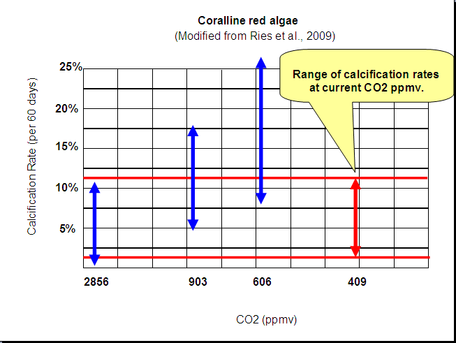
Fig. 5) Coralline red algae calcification response to increased atmospheric CO2 (modified after Ries eta la., 2009)

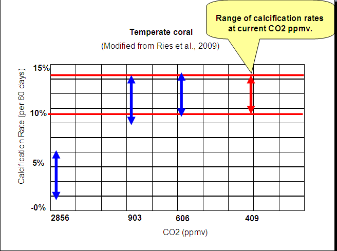
Fig. 6) Temperate coral calcification response to increased atmospheric CO2 (modified after Ries et al., 2009).

 

Neither coral species experienced negative effects to calcification rates at CO2 levels below 1,000 to 2,000 ppmv. The study reared the various species in experimental sea water using 4 different CO2 and aragonite saturation scenarios.

It appears that in addition to being plant food… CO2 is also reef food. 

More CO2 in the atmosphere leads to something called “CO2 fertilization.” In an enriched CO2 environment, most plants end to grow more. The fatal flaw of the infamous “Hockey Stick” chart was in Mann’s misinterpretation of Bristlecone Pine tree ring chronologies as a proxy for temperature; when in fact the tree ring growth was actually indicating CO2 fertilization as in this example from Greek fir trees…

Fig. 7) Example of CO2 fertilization in Greek fir trees (Koutavas, 2008 from CO2 Science)

Coral reefs can only grow in the photic zone of the oceans because zooxanthellae algae use sunlight, CO2, calcium and/or magnesium to make limestone.

The calcification rate of Flinders Reef has increased along with atmospheric CO2 concentrations since 1700…

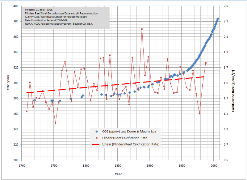
Fig. 8) Flinders Reef calcification rate plotted with atmsopheric CO2.

As the atmospheric CO2 concentration has grown since the 1700’s coral reef extension rates have also trended upwards. This is contrary to the theory that increased atmospheric CO2 should reduce the calcium carbonate saturation in the oceans, thus reducing reef calcification. It’s a similar enigma to the calcification rates of coccoliths and otoliths.

In all three cases, the theory or model says that increasing atmospheric CO2 will make the oceans less basic by increasing the concentration of H+ ions and reducing calcium carbonate saturation. This is supposed to reduce the calcification rates of carbonate shell-building organisms. When, in fact, the opposite is occurring in nature with reefs and coccoliths – Calcification rates are generally increasing. And in empirical experiments under laboratory conditions, otoliths grew (rather than shrank) when subjected to high levels of simulated atmospheric CO2.

In the cases of reefs and coccoliths, one answer is that the relatively minor increase in atmospheric CO2 over the last couple of hundred years has enhanced photosynthesis more than it has hampered marine carbonate geochemistry. However, the otoliths (fish ear bones) shouldn’t really benefit from enhanced photo-respiration. The fact that otoliths grew rather than shrank when subjected to high CO2 levels is a pretty good indication that the primary theory of ocean acidification has been tested and falsified.

Some may say, “Hey! That’s just one reef!  Flinders reef is an outlier!”  Fair point.  So let’s look at a larger data set. 

The January 2, 2009 issue of Science featured a paper, Declining Coral Calcification on the Great Barrier Reef, by Glenn De’ath, Janice M. Lough, Katharina E. Fabricius. This is from the abstract:

Reef-building corals are under increasing physiological stress from a changing climate and ocean absorption of increasing atmospheric carbon dioxide. We investigated 328 colonies of massive Porites corals from 69 reefs of the Great Barrier Reef (GBR) in Australia. Their skeletal records show that throughout the GBR, calcification has declined by 14.2% since 1990, predominantly because extension (linear growth) has declined by 13.3%. The data suggest that such a severe and sudden decline in calcification is unprecedented in at least the past 400 years.

I have not purchased the article and my free membership to the AAAS does not grant access to it; but I did find the database that appears to go with De’ath et al., 2009 in the NOAA Paleoclimatology library: LINK

Well… I downloaded the data to Excel and I calculated an annual average calcification rate for the 59 cores that are represented in the data set. This is what I came up with…

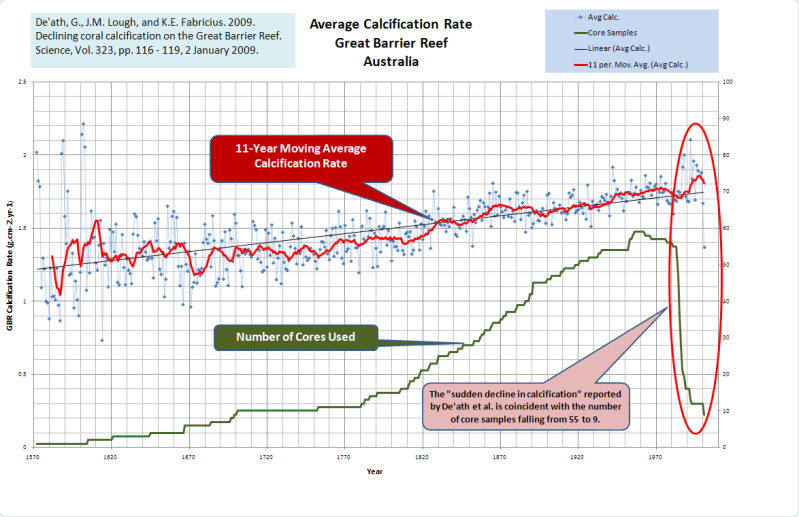
Fig. 9) Great Barrier Reef Calcification Rate (after De'ath et al., 2009)

It is “cherry-picking” of the highest order, if that last data point really is the basis of this claim: “Their skeletal records show that throughout the GBR, calcification has declined by 14.2% since 1990, predominantly because extension (linear growth) has declined by 13.3%. The data suggest that such a severe and sudden decline in calcification is unprecedented in at least the past 400 years.”

Over the last 400+ years the Earth’s climate has warmed ~0.6°, mean sea level has risen by about 9 inches and the atmosphere has become about 100 ppmv more enriched with CO2; and the Great Barrier Reef has responded by steadily growing faster.

1. Rising Temperature: The Great Barrier Reef likes the warm-up since the depths of the Little Ice Age…

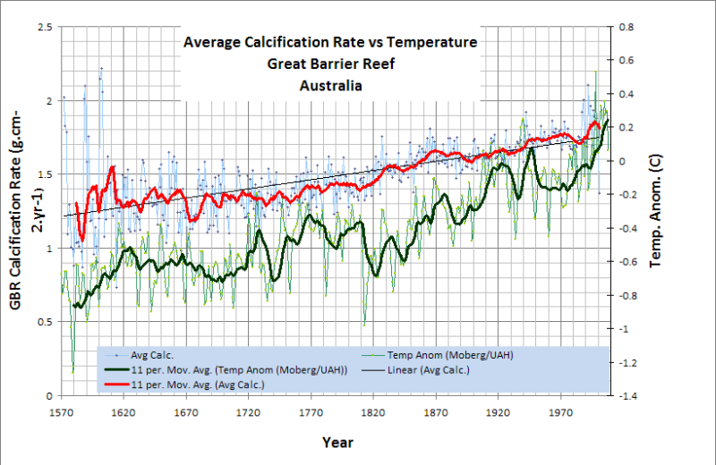
Fig. 10) GBR calcification rate and temperature.

2. Rising Sea Level: The Great Barrier Reef likes the slight sea level rise since the depths of the Little Ice Age…

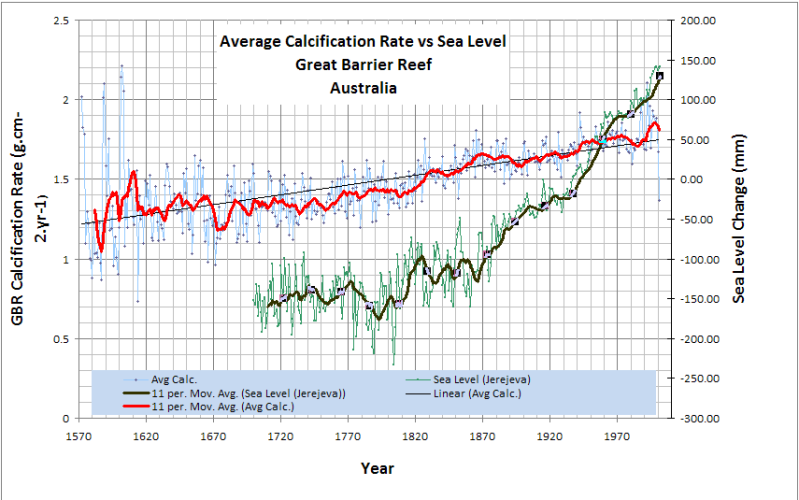
Fig. 11) GBR calcification rate and sea level.

3. Rising Atmospheric CO2 Concentrations: The Great Barrier Reef likes the increase in CO2 levels since the depths of the Little Ice Age…

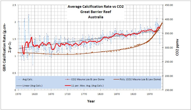
Fig. 12a) GBR calcification rate and atmsopheric CO2.

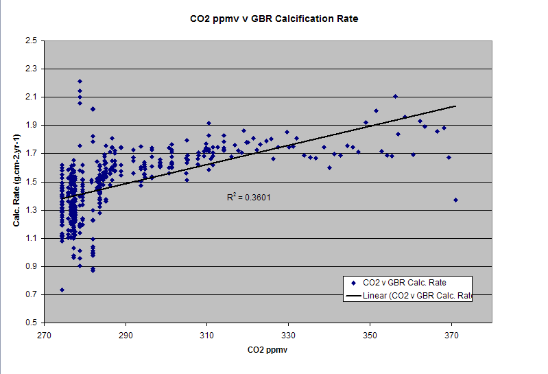
Fig. 12b) GBR calcification rate and atmospheric CO2 cross plot.

 

Does the geological record support the oceanic acidification hypothesis?

Average annual pH reconstructions and measurements from various Pacific Ocean locations:

60 million to 40 million years ago: 7.42 to 8.04 (Pearson et al., 2000)
23 million to 85,000 years ago: 8.04 to 8.31 (Pearson et al., 2000)
6,000 years ago to present: 7.91 to 8.28 (Liu et al., 2009)
1708 AD to 1988 AD: 7.91 to 8.17 (Pelejero et al., 2005)
2000 AD to 2007 AD: 8.10 to 8.40 (Wootton et al., 2008)

The low pH levels from 60 mya to 40 mya include the infamous Paleocene-Eocene Thermal Maximum (PETM). E ven then, the oceans did not actually “acidify;” the lowest pH was 7.42 (still basic).

The Paleocene-Eocene Thermal Maximum (PETM) was a period of significant global warming approximately 55 million years ago and has often been cited as a geological analogy for the modern threat of ocean acidification. There is solid evidence that the Lysocline “shoaled” or became shallower for a brief period of time during the PETM. Several cores obtained from the Walvis Ridge area in the South Atlantic during Ocean Drilling Program (ODP) Leg 208 contained a layer of red clay at the P-E boundary in the middle of an extensive carbonate ooze section (Zachos et al., 2005). This certainly indicates a disruption of the lysocline during the PETM; but it doesn’t prove that it was ocean acidification.

The PETM was a period of extensive submarine and subaerial volcanic activity (Storey et al., 2007) and pedogenic carbonate reconstructions do support the possibility that seafloor methane hydrates released by that volcanic activity may have sharply increased oceanic CO2 saturation.

But… The terrigenous paleobotanical evidence does not support elevated atmospheric CO2 levels during the PETM (Royer et al., 2001). The SI data indicate CO2 levels in North America to have been between 300 and 400 ppmv during the PETM.

So, the PETM may have been an example of ocean acdification… But there is NO evidence that it was caused by a sharp increase in atmospheric CO2 levels.

The range of oceanic pH variation over the last 200 years is well within the natural variation range over the last 7,000 years.

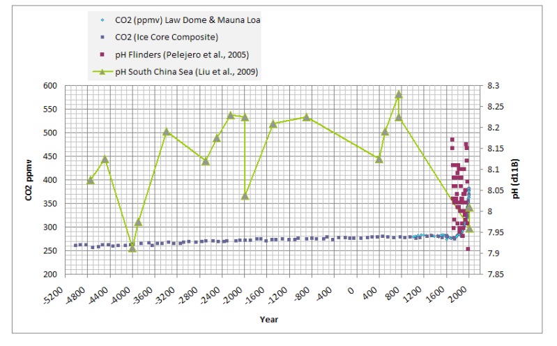
Fig. 13) 7,000 years of pH and atmospheric CO2

Some have asserted that there is no geological precedent; claiming atmospheric CO2 concentrations have risen faster in the last 150 years than at any time in recent geological history.  Ice core-derived CO2 data certainly do indicate that CO2 has not risen above ~310 ppmv at any point in the last 600,000 years and that it varies little at the decade or century scale.  However, there are other methods for estimating past atmospheric CO2 concentrations. 

Plants “breath” CO2 through microscopic epidermal pores called stomata.  The density of plant stomata varies inversely with the atmospheric partial pressure of CO2.  Several recent studies of plant stomata from living, herbarium and fossil samples of plant tissue have shown that atmospheric CO2 fluctuations comparable to that seen in the industrial era have been fairly common throughout the Holocene and Recent times.

Plant stomata measurements reveal large variations in atmospheric CO2 concentrations over the tast 2,000 years that are not apparent in ice core data (Kouwenberg, 2004)…

Fig. 14) Kouwenberg (2004) Figure 5.4: Reconstruction of paleo-atmospheric CO2 levels when stomatal frequency of fossil needles is converted to CO2 mixing ratios using the relation between CO2 and TSDL as quantified in the training set. Black line represents a 3 point running average based on 3–5 needles per depth. Grey area indicates the RMSE in the calibration. White diamonds are data measured in the Taylor Dome ice core (Indermühle et al., 1999); white squares CO2 measurements from the Law Dome ice-core (Etheridge et al., 1996). Inset: Training set of TSDL response of Tsuga heterophylla needles from the Pacific Northwest region to CO2 changes over the past century (Chapter 4).

Century-scale fluctuations in atmospheric CO2 concentrations have also been demonstrated in the early Holocene (Wagner et al., 1999)…

Fig. 15) (Wagner et al., 1999) Fig. 1. (A) Mean SI values (±1 ) for B. pendula and B. pubescens from the early Holocene part of the Borchert section (Netherlands; 52.23°N, 7.00°E) and reconstructed CO2 concentrations. The scale of the section is in centimeters. Three lithological (Lith.) units can be recognized (18): a basal gyttja (=), succeeded by Drepanocladus peat (//), which is subsequently overlain by Sphagnum peat ( ). Six conventional 14C dates (in years before the present) are available (indicated by circled numbers): 1, 10,070 ± 90; 2, 9930 ± 45; 3, 9685 ± 90; 4, 9770 ± 90; 5, 9730 ± 50; and 6, 9380 ± 80. Summary pollen diagram includes arboreal pollen (white area) with Pinus ( ) and with Betula ( ) and nonarboreal pollen with Gramineae ( ) and with Cyperaceae, upland herbs, and Ericales ( ). Regional climatic phases after (18): YD, Younger Dryas; Fr., Friesland phase; Ra., Rammelbeek phase; and LP, Late Preboreal. For analytical method, see (13). Quantification of CO2 concentrations according to the rate of historical CO2 responsiveness of European tree birches (Fig. 2). P indicates the reconstructed position of the Preboreal Oscillation.

If the plant stomata data are correct, the increase in atmospheric CO2 that has occurred over the last 150 years is not anomalous. Past CO2 increases of similar magnitude and rate have not caused ocean acidification.  In fact, marine calcifers would probably take 3,000 ppmv CO2 in stride, just by making more limestone… Kind of like they did during the Cretaceous…

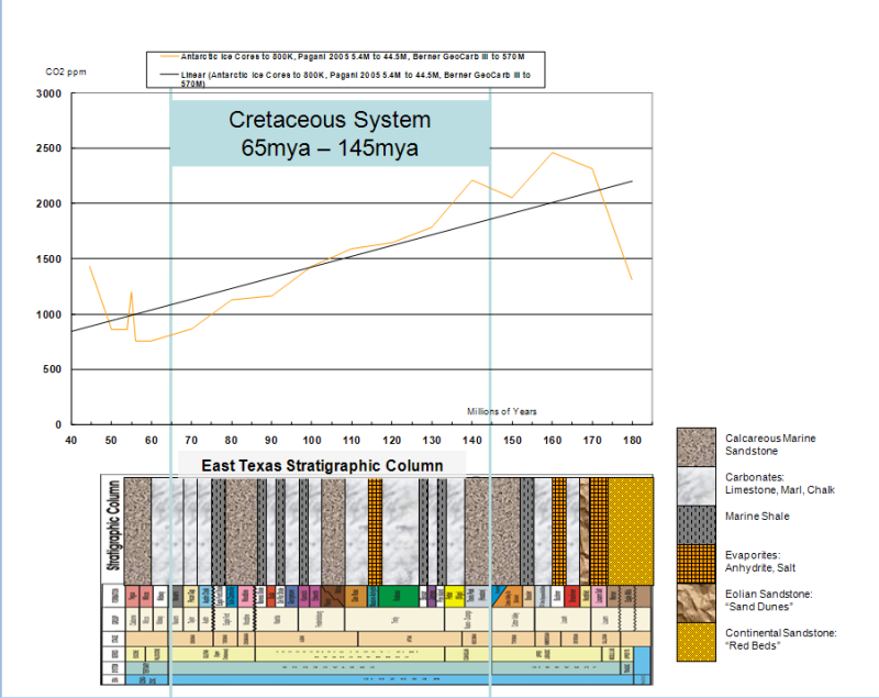
Fig. 16) East Texas Stratigraphic Column and Creatceous CO2

Once again, we have an environmental catastrophe that is entirely supported by predictive computer models and totally unsupported by correlative and empirical scientific data.  We can safely pitch ocean acidification into the dustbin of junk science.  

References

Reef data from:

De’ath, G., J.M. Lough, and K.E. Fabricius. 2009.
Declining coral calcification on the Great Barrier Reef.
Science, Vol. 323, pp. 116 – 119, 2 January 2009.

Lough, J.M. and D.J. Barnes, 2000.
Environmental controls on growth of the massive coral Porites.
Journal of Experimental Marine Biology and Ecology, 245: 225-243.

Lough, J.M. and D.J. Barnes, 1997.
Several centuries of variation in skeletal extension, density and calcification in massive Porites colonies from the Great Barrier Reef: a proxy for seawater temperature and a background of variability against
which to identify unnatural change.
Journal of Experimental Marine Biology and Ecology, 211: 29-67.

Chalker, B.E. and D.J. Barnes, 1990.
Gamma densitometry for the measurement of coral skeletal density.
Coral Reefs, 4: 95-100.

Temperature data from:

Moberg, A., D.M. Sonechkin, K. Holmgren, N.M. Datsenko and W. Karlén. 2005.
Highly variable Northern Hemisphere temperatures reconstructed from low-and high-resolution proxy data.
Nature, Vol. 433, No. 7026, pp. 613-617, 10 February 2005.

University of Alabama, Hunstville

Sea Level data from:

“Recent global sea level acceleration started over 200 years ago?”, Jevrejeva, S., J. C. Moore, A. Grinsted, and P. L. Woodworth (2008), Geophys. Res. Lett., 35, L08715, doi:10.1029/2008GL033611.

CO2 data from:

D.M. Etheridge, L.P. Steele, R.L. Langenfelds, R.J. Francey, J.-M. Barnola and V.I. Morgan. 1998. Historical CO2 records from the Law Dome DE08, DE08-2, and DSS ice cores. In Trends: A Compendium of Data on Global Change. Carbon Dioxide Information Analysis Center, Oak Ridge National Laboratory, U.S. Department of Energy, Oak Ridge, Tenn., U.S.A.

Dr. Pieter Tans, NOAA/ESRL (www.esrl.noaa.gov/gmd/ccgg/trends)

Other references:

Royer, et al., 2001. Paleobotanical Evidence for Near Present-Day Levels of Atmospheric CO2 During Part of the Tertiary. Science 22 June 2001: 2310-2313. DOI:10.112

Caldeira, K. and Wickett, M.E. 2003. Anthropogenic carbon and ocean pH. Nature 425: 365.

Orr, J.C., et al., 2005. Anthropogenic ocean acidification over the twenty-first century and its impact on calcifying organisms. Nature 437, 681-686 (29 September 2005) | doi:10.1038

Pelejero, C., Calvo, E., McCulloch, M.T., Marshall, J.F., Gagan, M.K., Lough, J.M. and Opdyke, B.N. 2005. Preindustrial to modern interdecadal variability in coral reef pH. Science 309: 2204-2207.

Zachos, et al., 2005. Rapid Acidification of the Ocean During the Paleocene-Eocene Thermal Maximum . Science 10 June 2005: 1611-1615. DOI:10.1126

Storey, et al., 2007. Paleocene-Eocene Thermal Maximum and the Opening of the Northeast Atlantic. Science 27 April 2007: 587-589. DOI:10.1126

Late 20th-Century Acceleration in the Growth of Greek Fir Trees. Volume 11, Number 49: 3 December 2008, CO2 Science

Iglesias-Rodriguez, et al., 2008. Phytoplankton Calcification in a High-CO2 World. Science 18 April 2008: 336-340 DOI:10.1126

Koutavas, A. 2008. Late 20th century growth acceleration in greek firs (Aibes cephalonica) from Cephalonia Island, Greece: A CO2 fertilization effect? Dendrochronologia 26: 13-19.

The Ocean Acidification Fiction. Volume 12, Number 22: 3 June 2009, CO2 Science

Checkley, et al., 2009. Elevated CO2 Enhances Otolith Growth in Young Fish. Science 26 June 2009: 1683. DOI:10.1126

Liu, Y., Liu, W., Peng, Z., Xiao, Y., Wei, G., Sun, W., He, J. Liu, G. and Chou, C.-L. 2009. Instability of seawater pH in the South China Sea during the mid-late Holocene: Evidence from boron isotopic composition of corals. Geochimica et Cosmochimica Acta 73: 1264-1272.

Ries, J.B., A.L. Cohen, D.C. McCorkle.  Marine calcifiers exhibit mixed responses to CO₂-induced ocean acidification.  Geology 2009 37: 1131-1134.